
- skin lesion classification
- dermoscopy
- ISIC2018
- ResNet50
- attention mechanism
- dual branch network
- global local attention
- medical image AI
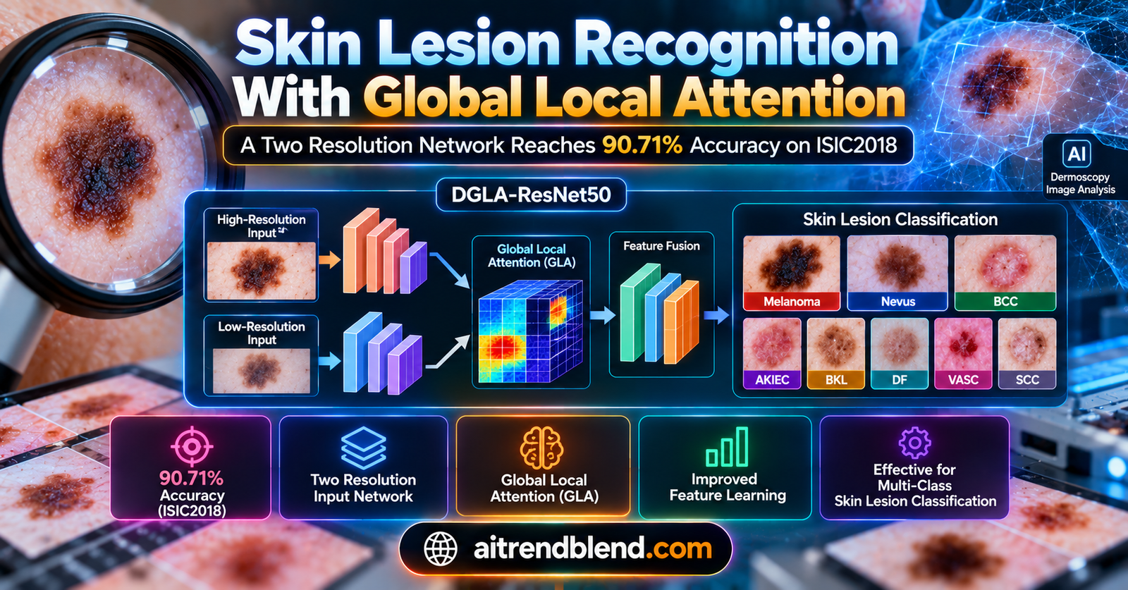
A dermatologist bends over a dermoscope and studies a brown patch no bigger than a pencil eraser on a patient’s back. Is it an ordinary mole, an early melanoma, or a benign keratosis that only pretends to be dangerous? Human experts disagree on cases like this more often than most patients would like to believe, and the number of images keeps growing.
That is the clinical setting behind a 2024 paper in Engineering Applications of Artificial Intelligence, where Ling Tan, Hui Wu, Jingming Xia, Ying Liang and Jining Zhu at Nanjing University of Information Science and Technology build a classifier for seven and eight types of skin lesion. Their network, DGLA-ResNet50, reaches 90.71% accuracy on ISIC2018 while adding attention in a deliberately cheap way. It is a useful piece of engineering. It is also a paper whose headline claims deserve a slower read than the abstract invites, and that slower read is what follows.
Key points
- DGLA-ResNet50 reaches 90.71% accuracy on ISIC2018 with seven lesion classes and 87.24% on ISIC2019 with eight classes.
- Every image is processed at 224 by 224 and at 448 by 448 pixels by two weight sharing branches that fuse three times along the way.
- Horizontal attention followed by vertical attention lets each pixel see the whole image indirectly, at a small fraction of full self attention cost.
- Melanoma precision on ISIC2018 is only 71.36%, the weakest of the seven classes, so the headline accuracy hides the hardest cases.
- The lightweight label is relative. FLOPs rise from 3.9G to 15.6G against plain ResNet50, and CI-Net still scores higher accuracy at 94.62%.
- No code is released, results come from a single split, and no confidence intervals are given, so this is a research result and not a clinical tool.
Please read this first. This article explains published research. It is not medical advice, diagnosis or treatment. Any change in a mole or patch of skin should be examined by a qualified dermatologist or physician.
Why dermoscopy images resist simple classifiers
The problem runs deeper than it first appears. Dermoscopy magnifies a lesion, but it does not decide anything. The public ISIC2018 collection, which the authors use as a seven class benchmark, contains 10,015 images. Of those, 6,705 show melanocytic nevi, about two thirds of everything, while dermatofibroma has just 115 examples and vascular lesions 142. A network trained naively on that mix can look accurate simply by guessing the common class.
Then there is the visual side. A lesion may fill the frame or sit in a small corner. Two patients with the same diagnosis can present lesions that look nothing alike, which researchers call intra class variation, and two different diagnoses can look almost identical, which is inter class similarity. Both problems get worse when training data is thin, and medical datasets are almost always thin.
Early computer aided systems relied on hand crafted features. Alencar and colleagues (2016) fed asymmetry, border, color and diameter measurements into a multilayer perceptron, while Kasmi and Mokrani (2016) removed hair with a Gabor filter, traced lesion boundaries with geodesic active contours and then applied the ABCD rule. Those pipelines need expert guidance at every step, and a wrong choice early on loses information for good.
Deep networks removed much of the hand tuning. Yu and colleagues (2016) stacked more than fifty residual layers for melanoma recognition, and Hosny and colleagues (2020) adapted AlexNet through transfer learning for seven classes. Depth helped, but it also piled up parameters and slowed recognition, a tension that runs through the rest of this paper. Zhang and colleagues (2019) then argued that residual networks suit medical images better than several alternatives, partly because shortcut connections keep the parameter count modest on small datasets. That argument is why Tan and colleagues chose ResNet50 as their backbone.
Where global attention becomes expensive
Attention modules are the usual answer to lesions that vary in size and position. Squeeze and excitation blocks (Hu et al., 2018) and CBAM (Woo et al., 2018) are popular in skin disease work, yet the authors argue that they lean on simple pooling to condense global context, and pooling throws away detail. Tiny lesions inside highly similar images are exactly where that loss hurts.
Self attention keeps more information but charges more for it. The non local block (Wang et al., 2018) multiplies large matrices, and on a large feature map the memory bill becomes painful. CCNet (Huang et al., 2019) trimmed the cost by letting each query look at fewer points, and Nakai and colleagues (2022) tried an enhanced bottleneck transformer for skin lesions, which the paper says still carries high computational complexity.
Here is a way to picture the trade. Imagine a stadium crowd trying to share one message. Full self attention asks every person to shout at every other person, which is deafening. The approach in this paper asks each person to pass the message along their row, and then asks everyone to pass along whatever they heard up and down their column. Two quiet hops, and the whole stadium has heard it, at least indirectly. That is the heart of the horizontal vertical attention idea, and it sits much closer to criss cross designs such as CCNet than to a full transformer.
Two zoom levels through the dual branch input network
One image, two resolutions, shared weights
The dual branch input network, or DBI, starts from a simple observation. A single fixed resolution suits some lesions and fails others. So the authors prepare every image twice. Each dermoscopy image is padded with black pixels into a 600 by 600 square, then shrunk to 224 by 224 for the main branch and to 448 by 448 for a second branch that supplies extra multi scale information.
In Figure 1 of the paper the two branches run the same GLA-ResNet50 stages side by side. After the first, second and third stage the feature maps are concatenated, squeezed back down with a 1 by 1 convolution and added into the main branch before the next stage begins. Only the main branch produces the final class scores.
Two full networks would double the cost, so the authors share parameters between the branches. That decision explains a curious line in their ablation table. Adding the DBI to plain ResNet50 lifts the parameter count from 90M to only 91.3M, yet FLOPs climb from 3.9G to 6.7G, because the larger 448 pixel input still has to be pushed through the shared layers. Weights are cheap to share. Computation is not.
The payoff on ISIC2018 is 1.33 accuracy points, from 83.26% to 84.59%. On ISIC2019 it is 1.31 points, from 78.35% to 79.66%. Real, but modest.
What the paper leaves unsaid about alignment
Here is a detail worth pausing on. The text says the peer stages of both branches output feature maps of the same size before concatenation. Table 1 in the paper lists a 56 by 56 map after the second stage for a 224 pixel input. A 448 pixel input would naturally produce a 112 by 112 map at that same stage. How the two are matched, whether by pooling, strided convolution or something else, is not described.
It is a small omission with a big consequence for anyone trying to reproduce the result. It is also why the code later in this article marks its own choice clearly as an assumption.
Global local attention, piece by piece
The global local attention module, or GLA, is where most of the design effort went. It has a global path built from horizontal attention followed by vertical attention, and a local path built from three ordinary convolutions. The outputs are added to the input feature map inside a ResNet bottleneck.
Horizontal attention and why it costs so little
Start with a feature map X that has C channels, height H and width W. Two 1 by 1 convolutions produce a query map Q and a key map K, both with a reduced channel count \(C_1\). A third produces a value map V that keeps all C channels. Three economies follow.
- Fewer channels. Queries and keys use \(C_1\) channels, which the authors require to be smaller than C.
- Fewer queries. The query map is resized to half its height and width, so only a quarter of the positions ask questions.
- Fewer keys. Each query compares itself only with the W keys in its own row, and not with every position in the image.
For each query vector the module takes a dot product with every key in that row. The result is a horizontal dependency score for each column.
A softmax over those W scores gives the attention map. The value map is averaged along its height, leaving one representative vector per column, and the attention map mixes those vectors.
The result is resized back to full resolution, scaled by a learnable weight alpha, and added to X.
That weight starts at zero, and the start matters. At the first training step the module does nothing at all, and the network is free to decide how much horizontal context it wants.
How much is actually saved? Take a 56 by 56 feature map, the size after the first ResNet stage. Full self attention needs 3,136 times 3,136 pairwise scores, which is 9,834,496. With half resolution queries that each inspect one row of 56 keys, the module needs 28 times 28 times 56 scores, which is 43,904. This is my own back of the envelope arithmetic from the shapes in the paper, not a figure the authors report, and it ignores the convolutions and the aggregation step. Still, a reduction of about 224 times in the affinity computation, exactly four times the map height, explains why the authors call the module lightweight.
None of this comes for free. Averaging values over the height is a lossy step, because each attention weight chooses among column averages and not among individual pixels. Fine vertical detail inside a column is blurred before the mix. The paper also does not say which key row a half resolution query is matched with, so every implementation has to pick a convention.
Vertical attention and the two hop trick
Vertical attention is the same machine turned on its side. Queries compare against the H keys in their own column, values are averaged along the width, and a second learnable weight, beta, starts at zero. On its own, horizontal attention only connects pixels that share a row, and vertical attention only connects pixels that share a column.
The authors chain them. Horizontal attention runs first and produces a map called I1. Vertical attention then runs on I1 and produces I2. Think about what this actually achieves. Take any two pixels, m and q. If they share a row or a column, one module connects them directly. If they do not, information from q first travels along its row to the pixel that sits in the same column as m, and then along that column to m. Figure 5 in the paper walks through all three cases.
Two cheap passes reach every position, which is why the authors say global information is obtained indirectly.
KEY TAKEAWAYRow then column attention buys global context in two cheap hops. The price is that the context is indirect and built from pooled values, so it is a compressed view of the image and not a faithful copy of full self attention.
Local attention from three plain convolutions
The local path is almost disappointingly simple. Three 3 by 3 convolutions in a row turn the feature map into a new map called X prime. A softmax is then applied across all spatial positions of each channel, and the result multiplies the original features.
There is a subtle point here. A softmax over spatial positions produces weights that sum to one for every channel, so on a 56 by 56 map the average weight is about one in 3,136. The gate can still sharpen wherever the convolutions produce large values, and the learnable scale on the local branch can grow to compensate, but the raw magnitude of this path starts very small. The paper does not discuss how this behaves during training, which is a fair question to put to the authors.
How the pieces meet inside a bottleneck
Inside the GLA Bneck block, a 1 by 1 convolution reduces channels, the GLA module takes the place of the usual 3 by 3 convolution, and a second 1 by 1 convolution restores the channels before the residual addition. Batch normalization and ReLU follow the familiar pattern. Stacking these blocks in the standard 3, 4, 6 and 3 layout gives GLA-ResNet50, and running two copies with fusion gives DGLA-ResNet50.
Equations 9 to 11 in the paper combine the global and local paths with the input.
Read literally, the identity map X enters twice, once directly in the first equation and once inside the global term of the second. Because alpha and beta start at zero this is probably harmless in practice, and it may be a notational slip, but without released code there is no way to check. The PyTorch version below keeps the equations as written and exposes a switch for the single identity variant.
What the experiments actually show
Datasets and the training recipe
The authors test on two public collections. ISIC2018 has 10,015 dermoscopy images in seven categories, and ISIC2019 has 25,331 images in eight, the extra one being squamous cell carcinoma, which arrived with the BCN20000 data. For ISIC2019 they train on 22,000 images and test on 3,331. The paper does not state the ISIC2018 split, but the confusion matrix in its Figure 7 adds up to roughly 2,003 test images, which would be about one fifth of the data.
Class imbalance is handled with weighted random sampling, which draws rare classes more often during training. For the comparison against other networks, every model was trained from scratch with the same settings, an initial learning rate of 0.0001, stochastic gradient descent and a batch size of 8. That keeps the comparison even. It also means none of the models benefit from pretraining, which other work cited in the paper, such as Hosny and colleagues (2020), does rely on, so the absolute numbers are not directly comparable with pretrained systems elsewhere. The paper also leaves out the number of epochs, the loss function and the augmentation settings for the main experiments.
The ablation story
Table 1 reproduces the paper’s ablation. Each module helps. On ISIC2018 the DBI adds 1.33 points, the GLA module adds 4.46, and the two together add 7.45, moving accuracy from 83.26% to 90.71%. On ISIC2019 the increments are 1.31, 6.68 and 8.89 points.
| Model | ISIC2018 accuracy (%) | ISIC2019 accuracy (%) | Params ISIC2018 (M) | Params ISIC2019 (M) | FLOPs (G) |
|---|---|---|---|---|---|
| ResNet50 | 83.26 | 78.35 | 90 | 137.2 | 3.9 |
| DBI-ResNet50 | 84.59 | 79.66 | 91.3 | 153.1 | 6.7 |
| GLA-ResNet50 | 87.72 | 85.03 | 101.3 | 176.7 | 12.4 |
| DGLA-ResNet50 | 90.71 | 87.24 | 104.2 | 189.3 | 15.6 |
Table 1. Ablation of the two modules, values as reported by Tan et al. (2024).
The paper also splits the GLA module into its two paths. Adding only horizontal vertical attention to ResNet50 gives 85.01% on ISIC2018, up 1.75 points, for 8.5M extra parameters. Adding only the local path gives 84.37%, up 1.11 points, for just 2.6M extra. Combined they reach 87.72%, which is more than the sum of the parts. On ISIC2019 the picture flips. The two separate gains of 4.27 and 2.89 points add up to more than the 6.68 the combination achieves. So the paths look complementary on one dataset and partly redundant on the other, a nuance the paper’s prose glosses over. One small arithmetic point too. The text quotes a 4.24 point gain for horizontal vertical attention on ISIC2019, while Table 5 of the paper implies 4.27.
Head to head with other networks
The paper compares six other networks, all trained from scratch under the same settings. Table 2 shows the ISIC2018 results.
| Model | Accuracy (%) | Average precision (%) | Weighted precision (%) | Weighted F1 (%) | Params (M) | FLOPs (G) |
|---|---|---|---|---|---|---|
| Inception V4 | 81.53 | 81.07 | 84.15 | 82.82 | 146.9 | 26.8 |
| ResNet101 | 84.01 | 81.16 | 84.29 | 84.14 | 164.5 | 7.9 |
| ARL-CNN50 | 85.03 | 86.47 | 89.67 | 87.29 | 95.7 | 8.6 |
| DABN-ELW | 88.79 | 87.65 | 88.04 | 88.41 | 286.3 | 31.1 |
| Eff2Net | 85.78 | 84.17 | 86.32 | 86.05 | 96.4 | 13.6 |
| CI-Net | 94.62 | 87.11 | 89.76 | 92.13 | 172.4 | 21.2 |
| DGLA-ResNet50 | 90.71 | 88.13 | 91.39 | 91.05 | 104.2 | 15.6 |
Table 2. Comparison on ISIC2018, values as reported by Tan et al. (2024).
DGLA-ResNet50 posts the best average precision at 88.13% and the best weighted precision at 91.39%, plus the second best accuracy and weighted F1. The accuracy leader is CI-Net at 94.62%. The authors call the gap slight and point to lower cost as compensation, since DGLA-ResNet50 uses 68.2M fewer parameters and 5.6G fewer FLOPs.
The numbers tell a complicated story. DGLA-ResNet50 misclassifies about 9.3% of the test images and CI-Net about 5.4%, so the smaller model makes roughly 1.7 times as many mistakes. There is a curious pattern as well. CI-Net leads on accuracy and weighted F1 but trails on average precision, which treats every class equally. The two metrics reward different behavior, and the paper reports no per class recall that would settle which system is better on the lesions that matter most. Against ARL-CNN50, the closest match in size, DGLA-ResNet50 gains 5.68 accuracy points for 8.5M more parameters, which is a good trade.
“DGLA-ResNet50 can improve the accuracy well while ensuring the lightweight of the model”
Tan et al., abstract of the source paper
Class by class precision
Overall accuracy hides where the errors live. Table 3 shows precision per class on ISIC2018. Nevus reaches 96.70% while melanoma sits at 71.36% and benign keratosis at 77.93%. DGLA-ResNet50 is also not uniformly the best. GLA-ResNet50 alone does better on benign keratosis at 84.31%, and plain ResNet50 beats the full model on vascular lesions, 94.20% against 93.10%.
| Model | MEL | NV | BCC | AKIEC | BKL | DF | VASC |
|---|---|---|---|---|---|---|---|
| ResNet50 | 62.27 | 91.33 | 66.82 | 83.33 | 75.28 | 90.48 | 94.20 |
| DBI-ResNet50 | 67.09 | 93.24 | 63.95 | 90.23 | 82.09 | 93.86 | 95.58 |
| GLA-ResNet50 | 70.75 | 94.48 | 80.12 | 87.50 | 84.31 | 94.74 | 89.66 |
| DGLA-ResNet50 | 71.36 | 96.70 | 88.64 | 94.44 | 77.93 | 94.74 | 93.10 |
Table 3. Precision per class (%) on ISIC2018. MEL melanoma, NV melanocytic nevus, BCC basal cell carcinoma, AKIEC actinic keratosis, BKL benign keratosis, DF dermatofibroma, VASC vascular lesion. Source Tan et al. (2024).
The confusion matrix in Figure 7 of the paper adds detail. It contains 1,339 nevus images out of roughly 2,003, about 67%, so a lazy classifier that always answered nevus would already look decent on accuracy. Among the melanoma images, 204 by my count of that row, 157 were classified correctly, 33 were labeled nevus and 12 benign keratosis. Actinic keratosis fared worse, with 51 of 83 found and 19 of the misses sent to benign keratosis. The authors themselves note that many categories get pulled toward nevus because of the imbalance.
Is it really lightweight?
Read the ablation table again. Plain ResNet50, in the paper’s accounting, has 90M parameters and 3.9G FLOPs. DGLA-ResNet50 has 104.2M and 15.6G, which is four times the computation for a 14.2M parameter increase. Against other attention modules the story looks better, as Table 4 shows.
| Model on ISIC2018 | Accuracy (%) | Params (M) | FLOPs (G) |
|---|---|---|---|
| ResNet50 with SE | 83.58 | 96.4 | 8.9 |
| ResNet50 with BAM | 84.10 | 94.7 | 8.6 |
| ResNet50 with CBAM | 84.99 | 96.9 | 9.3 |
| CCNet | 83.67 | 273.6 | 32.7 |
| GLA-ResNet50 (single input) | 87.72 | 101.3 | 12.4 |
Table 4. Attention methods compared on ISIC2018, values as reported by Tan et al. (2024).
So the honest reading is that GLA is cheaper than heavy attention and more accurate than cheap attention. That is a real result. But lightweight is relative to the comparison set, not to the baseline. One more oddity is that the parameter counts themselves look large for a ResNet50 family model, and the paper does not explain how it counts parameters or what its classification head and input pipeline add. Treat the parameter columns as comparisons inside the paper and not as absolute figures.
The authors also test their lightening tricks. Swapping the lightweight horizontal attention for a plain non local design, called NL-ResNet50, changes ISIC2018 accuracy from 88.23% to 87.72%, so the lightweight version gives up 0.51 points. On ISIC2019 the gap is larger at 1.88 points, 86.91% against 85.03%. The figure reports only score style metrics and no measured memory or runtime savings, so the trade cannot be priced from the paper alone. The F-ResNet50 numbers in that figure also match the GLA-ResNet50 row in the main tables, which suggests the comparison ran inside the full GLA setup even though the text describes a bare ResNet50 with one horizontal module.
What Grad-CAM and small data tests add
Two smaller experiments round out the evidence. The Grad-CAM heat maps in Figure 13 show GLA-ResNet50 focusing on the lesion despite hair, large lesions, tiny lesions and pale ones. They are persuasive as pictures. But the examples are few and there is no quantitative overlap measure against lesion outlines, so they work as illustration and not as proof.
The training size test in Table 8 is more informative. With 5,000 training images the model scores 88.97% accuracy and an AUC of 92.8. With the full 10,015 it reaches 90.71% and 94.6. With 15,000 images, built by adding translated and rotated copies of 4,985 images, it reaches 92.24% and 95.1. Performance falls gently as data shrinks, which supports the small sample claim. The 15,000 image case deserves caution though. If augmented copies of a test image ended up in training, the score would be inflated, and the paper does not say how the split was handled.
KEY TAKEAWAYThe DBI and GLA modules each add a measurable gain, and together they lift ISIC2018 accuracy from 83.26% to 90.71%. Yet melanoma is still the weakest class by precision, and the best accuracy in the comparison belongs to a different network.
From benchmark score to clinic
Clinical translation gap
A benchmark is a controlled experiment, and a clinic is not. The images in ISIC2018 and ISIC2019 come from curated challenge collections, with lesions selected and labeled for the competition. A dermatologist sees whoever walks in, on devices of varying quality, with hair, ink marks, unusual body sites and lesions that fit none of the seven classes.
Neither dataset in the paper works as an independent external test, because the authors describe ISIC2019 as an expansion of ISIC2018. Doing well on a second dataset that overlaps the first tells us less than doing well on a hospital’s own images. The paper also reports no breakdown by age, sex, body site or skin tone, so whether the results hold for the full range of patients is simply unknown.
Accuracy is not the number a clinician needs
Missing a melanoma and mislabeling a harmless nevus have very different consequences, yet accuracy treats them alike, and weighted recall in this paper equals accuracy by construction. A clinician would want sensitivity and specificity per class, ideally with confidence intervals, plus some sense of how well the model’s confidence is calibrated. By the numbers in Figure 7, 47 of the 204 melanoma test images were assigned to another class. That is nearly one in four.
Regulatory and safety notes
Software that influences diagnosis is generally regulated as a medical device. Regulators expect prospective clinical validation, documented performance across patient groups and a plan for monitoring after deployment. Nothing in this paper is designed to meet those requirements, and the authors themselves frame data imbalance and interpretability as open problems. Any pilot use should keep a clinician in the loop, treat the output as a second opinion at most, and log disagreements for review.
Limitations, with the real numbers
None of the following makes the work bad. It makes the evidence thinner than the abstract suggests, and a careful reader should know where.
- Sample size. ISIC2018 testing involves about 2,003 images, and some classes are tiny. By my row counts dermatofibroma has 22 test images and vascular lesions 28. The 94.74% precision for dermatofibroma comes from 19 predictions, of which 18 were correct, so one extra mistake would move it by nearly five points.
- Statistical evidence. Results appear to be single runs on one split, with no confidence intervals, seeds or significance tests. Gaps of one or two points between attention variants cannot be judged.
- Dataset bias and splitting. The stated ISIC2018 size of 10,015 matches the HAM10000 collection the authors cite, and that collection is documented to hold more than one image of some lesions. If images of the same lesion land on both sides of a random split, accuracy rises artificially. The paper does not say whether the split was done by lesion or by patient.
- Generalization. There is no external validation on images from another institution. ISIC2019 is a second benchmark and not an independent site.
- Baselines. Every competitor was trained from scratch with one learning rate and a batch size of 8. A different tuning per model could reorder the table.
- Reproducibility. The data availability statement calls the data confidential even though ISIC collections are public, and no code repository is cited. Alignment between branches, the key row convention, the loss, the epoch count and the initial local weight are all unspecified.
- Small slips. The opening skin cancer incidence figures cite a source titled Colorectal cancer statistics, 2020, which looks like a citation error, so check those numbers before reusing them. The 4.24 against 4.27 point mismatch and the doubled identity term are minor by comparison.
What practitioners can take from this work
If you build medical imaging models, three ideas here travel well. Row then column attention with pooled values is a drop in way to add global context to almost any convolutional backbone. Feeding two resolutions through shared weights is a cheap way to add scale robustness. And a spatial softmax gate on a small convolution stack is a simple local attention you can try in an afternoon.
Before trusting any of it, I would test five things.
- Split by lesion or patient, never by image.
- Report per class sensitivity and specificity with confidence intervals, with melanoma first.
- Validate on images from a different institution and device.
- Compare against pretrained baselines, since that is how most real systems start.
- Measure real latency and memory, because FLOPs and parameters are only proxies.
For more on where this sits in our coverage, see the AI for medical imaging hub (link to be added by the site owner). Two sibling analyses may interest you. One covers MT-Net and retinal microvascular segmentation, and another looks at trustworthy breast tumor segmentation using AI uncertainty, which speaks directly to the calibration gap discussed above.
Conclusion
The core achievement of this paper is a practical recipe. Take a familiar ResNet50, swap its middle convolution for an attention block that spends far less than full self attention, and feed it the same image at two sizes. On ISIC2018 that recipe lifts accuracy from 83.26% to 90.71%, and the gain survives a second dataset, a training size test and comparisons with five other attention or backbone designs. For a team working with a few thousand images, that is a meaningful engineering result.
The conceptual shift is subtler. Most attention work asks how a pixel can look at everything. This paper asks how a pixel can hear about everything, through a short chain of cheap hops. Context becomes something you assemble, row then column, and not something you compute in one expensive shot. Pair that with a second view at a different scale and you get a model that trades a little fidelity for a lot of efficiency.
The idea should transfer. Histopathology tiles, retinal photographs, satellite scenes and industrial inspection images all share the same headaches, meaning small important regions, variation in scale and limited labels. Wherever a feature map is large and the budget is small, a row then column attention block deserves a trial. I would not promise the same gains, since the ablation already shows the two attention paths behaving differently across two datasets.
The remaining limitations are real. Melanoma precision of 71.36%, a single split, no confidence intervals, an unexplained parameter count, no released code and a strong competitor with higher accuracy all argue for restraint. The word lightweight fits the attention block better than it fits the whole network, which needs four times the FLOPs of its baseline.
The authors point to the right next steps. Better handling of class imbalance, evaluation on more datasets and the addition of professional medical knowledge, such as the seven point checklist for texture and shape features, would each address a weakness visible in the numbers above. I would add per class sensitivity, lesion level splits and external validation to that list, and I would love to see the code.
A network that can see the whole image cheaply is only the start. The harder part is proving that it looks at the right thing, for the right patient, in the right clinic.
Complete PyTorch implementation
The authors did not release code, so the listing below is my independent reconstruction from the paper’s description. It includes the horizontal and vertical attention modules, the local attention path, the GLA Bneck block, the shared weight dual branch network, weighted random sampling, a training loop, an evaluation function and a smoke test on dummy data.
Wherever the paper is silent, the code says ASSUMPTION in a comment. The main ones are the key row convention for half resolution queries, the average pooling used to align the 448 pixel branch, cross entropy as the loss, momentum of 0.9 and a starting value of zero for the local weight. Change them deliberately and report what you changed.
"""
DGLA-ResNet50, an independent PyTorch reconstruction from the description in
Tan et al. (2024), Engineering Applications of Artificial Intelligence 127, 107385.

The authors did not release code. Every choice the paper leaves open is marked
with the word ASSUMPTION so that you can change it deliberately.
"""
import torch
import torch.nn as nn
import torch.nn.functional as F
from torch.utils.data import DataLoader, TensorDataset, WeightedRandomSampler


# ----------------------------------------------------------------------------
# 1. Horizontal attention (HA) and vertical attention (VA)
# ----------------------------------------------------------------------------
class HorizontalAttention(nn.Module):
    """Each half resolution query attends to the W keys in its own row (Eq. 1 to 3)."""

    def __init__(self, channels, reduction=8):
        super().__init__()
        c1 = max(channels // reduction, 8)          # ASSUMPTION, paper only says C1 < C
        self.q = nn.Conv2d(channels, c1, 1)
        self.k = nn.Conv2d(channels, c1, 1)
        self.v = nn.Conv2d(channels, channels, 1)
        self.alpha = nn.Parameter(torch.zeros(1))   # initial value 0, as in the paper

    def forward(self, x):
        b, c, h, w = x.shape
        h2, w2 = max(h // 2, 1), max(w // 2, 1)
        q = F.interpolate(self.q(x), size=(h2, w2), mode="bilinear", align_corners=False)
        k = self.k(x)
        # ASSUMPTION, the paper does not say which key row a half resolution query uses.
        rows = (torch.arange(h2, device=x.device) * h // h2).long()
        k_row = k[:, :, rows, :]                              # B, C1, H2, W
        d1 = torch.einsum("bchx,bchw->bwhx", q, k_row)        # B, W, H2, W2  (Eq. 1)
        a1 = F.softmax(d1, dim=1).flatten(2)                  # B, W, H2*W2
        e = self.v(x).mean(dim=2)                             # B, C, W  (average over height)
        f = torch.einsum("bcw,bwn->bcn", e, a1)               # Eq. 2, F = E A'
        f = f.reshape(b, c, h2, w2)
        g1 = F.interpolate(f, size=(h, w), mode="bilinear", align_corners=False)
        return self.alpha * g1 + x                            # Eq. 3


class VerticalAttention(nn.Module):
    """Vertical attention is horizontal attention applied to the transposed map (Eq. 4 and 5)."""

    def __init__(self, channels, reduction=8):
        super().__init__()
        self.inner = HorizontalAttention(channels, reduction)   # its alpha plays the role of beta

    def forward(self, x):
        return self.inner(x.transpose(2, 3)).transpose(2, 3)


# ----------------------------------------------------------------------------
# 2. Local attention (LA) and the full GLA module
# ----------------------------------------------------------------------------
class LocalAttention(nn.Module):
    """Three 3x3 convolutions, then a spatial softmax per channel (Eq. 8 and 11)."""

    def __init__(self, channels):
        super().__init__()
        self.convs = nn.Sequential(                 # ASSUMPTION, no BN or ReLU between the convs
            nn.Conv2d(channels, channels, 3, padding=1),
            nn.Conv2d(channels, channels, 3, padding=1),
            nn.Conv2d(channels, channels, 3, padding=1),
        )

    def forward(self, x):
        b, c, h, w = x.shape
        gate = F.softmax(self.convs(x).flatten(2), dim=-1).reshape(b, c, h, w)
        return gate * x                             # F_L = phi(X') * X


class GLA(nn.Module):
    """Global local attention, Y = X + F_G + gamma * F_L (Eq. 9 and 10)."""

    def __init__(self, channels, reduction=8, double_identity=True):
        super().__init__()
        self.ha = HorizontalAttention(channels, reduction)
        self.va = VerticalAttention(channels, reduction)
        self.la = LocalAttention(channels)
        self.gamma = nn.Parameter(torch.zeros(1))   # ASSUMPTION, initial value 0
        self.double_identity = double_identity      # the paper's equations count X twice

    def forward(self, x):
        f_g = self.va(self.ha(x))                   # beta*G2 + (alpha*G1 + X)
        f_l = self.la(x)
        if self.double_identity:
            return x + f_g + self.gamma * f_l       # literal reading of Eq. 9
        return f_g + self.gamma * f_l               # identity counted once


# ----------------------------------------------------------------------------
# 3. GLA Bneck, the ResNet bottleneck with GLA in place of the 3x3 convolution
# ----------------------------------------------------------------------------
class GLABneck(nn.Module):
    expansion = 4

    def __init__(self, in_ch, mid_ch, stride=1, double_identity=True):
        super().__init__()
        out_ch = mid_ch * self.expansion
        self.conv1 = nn.Sequential(nn.Conv2d(in_ch, mid_ch, 1, bias=False),
                                   nn.BatchNorm2d(mid_ch), nn.ReLU(inplace=True))
        self.gla = GLA(mid_ch, double_identity=double_identity)
        self.post = nn.Sequential(nn.BatchNorm2d(mid_ch), nn.ReLU(inplace=True))
        # ASSUMPTION, stride 2 is done with average pooling after the attention.
        self.pool = nn.AvgPool2d(2) if stride == 2 else nn.Identity()
        self.conv3 = nn.Sequential(nn.Conv2d(mid_ch, out_ch, 1, bias=False), nn.BatchNorm2d(out_ch))
        self.short = nn.Identity()
        if stride != 1 or in_ch != out_ch:
            self.short = nn.Sequential(nn.AvgPool2d(stride) if stride == 2 else nn.Identity(),
                                       nn.Conv2d(in_ch, out_ch, 1, bias=False),
                                       nn.BatchNorm2d(out_ch))

    def forward(self, x):
        y = self.post(self.gla(self.conv1(x)))
        y = self.conv3(self.pool(y))
        return F.relu(y + self.short(x))


def make_stage(in_ch, mid_ch, blocks, stride, double_identity=True):
    layers = [GLABneck(in_ch, mid_ch, stride, double_identity)]
    layers += [GLABneck(mid_ch * 4, mid_ch, 1, double_identity) for _ in range(blocks - 1)]
    return nn.Sequential(*layers)


# ----------------------------------------------------------------------------
# 4. DGLA-ResNet50, the dual branch input network with shared weights
# ----------------------------------------------------------------------------
class DGLAResNet50(nn.Module):
    def __init__(self, num_classes=7, double_identity=True):
        super().__init__()
        self.stem = nn.Sequential(nn.Conv2d(3, 64, 7, 2, 3, bias=False), nn.BatchNorm2d(64),
                                  nn.ReLU(inplace=True), nn.MaxPool2d(3, 2, 1))
        self.stages = nn.ModuleList([
            make_stage(64, 64, 3, 1, double_identity),      # 256 channels
            make_stage(256, 128, 4, 2, double_identity),    # 512 channels
            make_stage(512, 256, 6, 2, double_identity),    # 1024 channels
            make_stage(1024, 512, 3, 2, double_identity),   # 2048 channels
        ])
        # Fusion after stages 1, 2 and 3 only: concatenate, then a 1x1 convolution.
        self.fuse = nn.ModuleList([
            nn.Sequential(nn.Conv2d(2 * c, c, 1, bias=False), nn.BatchNorm2d(c))
            for c in (256, 512, 1024)
        ])
        self.fc = nn.Linear(2048, num_classes)

    def forward(self, x_main, x_aux):
        m, a = self.stem(x_main), self.stem(x_aux)          # 224 view and 448 view, same stem
        for i, stage in enumerate(self.stages):
            m = stage(m)
            if i < 3:
                a = stage(a)                                # shared weights, no second network
                # ASSUMPTION, the paper says peer maps have the same size but not how.
                a_small = F.adaptive_avg_pool2d(a, m.shape[-2:])
                m = m + self.fuse[i](torch.cat([m, a_small], dim=1))
        return self.fc(torch.flatten(F.adaptive_avg_pool2d(m, 1), 1))


# ----------------------------------------------------------------------------
# 5. Preprocessing, sampling, loss
# ----------------------------------------------------------------------------
def pad_to_square_and_resize(img, size):
    """Pad a C,H,W tensor with black pixels to a square, then resize (paper uses 600x600 first)."""
    _, h, w = img.shape
    side = max(h, w)
    img = F.pad(img, (0, side - w, 0, side - h))
    return F.interpolate(img[None], size=(size, size), mode="bilinear", align_corners=False)[0]


def two_views(img, main=224, aux=448):
    return pad_to_square_and_resize(img, main), pad_to_square_and_resize(img, aux)


def make_weighted_sampler(labels):
    """Weighted random sampling (WRS), rarer classes are drawn more often."""
    labels = torch.as_tensor(labels)
    counts = torch.bincount(labels).float()
    weights = (1.0 / counts)[labels]
    return WeightedRandomSampler(weights, num_samples=len(labels), replacement=True)


# The paper does not name its loss. ASSUMPTION, plain cross entropy, since WRS handles imbalance.
criterion = nn.CrossEntropyLoss()


# ----------------------------------------------------------------------------
# 6. Training loop and evaluation
# ----------------------------------------------------------------------------
def train(model, loader, epochs=1, lr=1e-4, device="cpu"):
    model.to(device).train()
    # Paper reports SGD, lr 0.0001 and batch size 8. Momentum is an ASSUMPTION.
    opt = torch.optim.SGD(model.parameters(), lr=lr, momentum=0.9)
    for epoch in range(epochs):
        running = 0.0
        for x_main, x_aux, y in loader:
            x_main, x_aux, y = x_main.to(device), x_aux.to(device), y.to(device)
            opt.zero_grad()
            loss = criterion(model(x_main, x_aux), y)
            loss.backward()
            opt.step()
            running += loss.item() * y.size(0)
        print(f"epoch {epoch + 1}  loss {running / len(loader.dataset):.4f}")


@torch.no_grad()
def evaluate(model, loader, num_classes, device="cpu"):
    """Accuracy, per class precision and recall, weighted precision and F1, confusion matrix."""
    model.to(device).eval()
    cm = torch.zeros(num_classes, num_classes, dtype=torch.long)
    for x_main, x_aux, y in loader:
        pred = model(x_main.to(device), x_aux.to(device)).argmax(1).cpu()
        for t, p in zip(y, pred):
            cm[t, p] += 1
    tp = cm.diag().float()
    precision = tp / cm.sum(0).clamp(min=1)
    recall = tp / cm.sum(1).clamp(min=1)
    f1 = 2 * precision * recall / (precision + recall).clamp(min=1e-9)
    support = cm.sum(1).float()
    w = support / support.sum()
    return {
        "accuracy": (tp.sum() / cm.sum()).item(),        # equals weighted recall
        "avg_precision": precision.mean().item(),
        "weighted_precision": (w * precision).sum().item(),
        "weighted_f1": (w * f1).sum().item(),
        "per_class_precision": precision.tolist(),
        "per_class_recall": recall.tolist(),
        "confusion_matrix": cm,
    }


# ----------------------------------------------------------------------------
# 7. Smoke test on dummy data
# ----------------------------------------------------------------------------
if __name__ == "__main__":
    torch.manual_seed(0)
    n, k = 16, 7
    labels = torch.randint(0, k, (n,))
    imgs = [torch.rand(3, 90, 120) for _ in range(n)]           # small dummy images
    views = [two_views(im, main=64, aux=128) for im in imgs]    # small sizes keep the test fast
    data = TensorDataset(torch.stack([v[0] for v in views]),
                         torch.stack([v[1] for v in views]), labels)
    loader = DataLoader(data, batch_size=4, sampler=make_weighted_sampler(labels))

    model = DGLAResNet50(num_classes=k)
    print("parameters (M)", sum(p.numel() for p in model.parameters()) / 1e6)
    out = model(*next(iter(loader))[:2])
    assert out.shape == (4, k), out.shape
    train(model, loader, epochs=1)
    metrics = evaluate(model, DataLoader(data, batch_size=4), k)
    print("dummy accuracy", round(metrics["accuracy"], 3))
    print("smoke test passed")
The listing passed a syntax check, but the smoke test could not be executed in the environment used to write this article, so please run it once yourself before relying on the code. It checks output shapes, one training epoch and the evaluation function, and it says nothing about accuracy on real skin images.
Frequently asked questions
What is DGLA-ResNet50 and what does it classify?
DGLA-ResNet50 is a convolutional network from Tan and colleagues that combines a dual branch input, which processes each image at two resolutions, with a global local attention module inside a ResNet50 backbone. It classifies dermoscopy images into seven lesion types on ISIC2018 and eight on ISIC2019.
How accurate is DGLA-ResNet50 on ISIC2018 and ISIC2019?
The paper reports 90.71% accuracy on ISIC2018 and 87.24% on ISIC2019. Results come from a single split with no confidence intervals, and CI-Net reached a higher accuracy of 94.62% on ISIC2018 in the same comparison.
Can DGLA-ResNet50 diagnose skin cancer?
No. It is a research model tested on public benchmark images. It has no external clinical validation, no regulatory clearance, and melanoma precision on ISIC2018 is 71.36%. Any skin change should be examined by a qualified dermatologist.
How does horizontal vertical attention differ from full self attention?
Full self attention compares every position with every other position. Horizontal vertical attention lets each query look only along its own row, then a second pass looks along columns, so information still reaches every position indirectly at a much lower cost.
Why is melanoma precision lower than nevus precision?
Nevus images make up about two thirds of ISIC2018, so the model sees far more of them, and melanoma often looks similar to nevus. In the paper’s confusion matrix, 33 melanoma images were labeled as nevus. The authors name class imbalance as an unsolved problem.
Is code available for DGLA-ResNet50?
The paper does not cite a code repository and its data availability statement calls the data confidential. This article includes an independent PyTorch reconstruction, with every unspecified design choice marked as an assumption.
Read the source paper. Tan and colleagues, Engineering Applications of Artificial Intelligence, 2024. The authors do not cite a code repository.
Read the paper ISIC 2018 challenge report on arXivTan, L., Wu, H., Xia, J., Liang, Y., Zhu, J. (2024). Skin lesion recognition via global-local attention and dual-branch input network. Engineering Applications of Artificial Intelligence, 127, 107385. https://doi.org/10.1016/j.engappai.2023.107385
Works named in the text appear in the reference list of the source paper. This analysis is based on the published paper and an independent evaluation of its claims.
Pingback: Revolutionizing Medical Image Segmentation: SemSim's Semantic Breakthrough - aitrendblend.com
Pingback: Revolutionizing Unsupervised Domain Adaptation: Cross-Modal Knowledge Distillation (CMKD) - aitrendblend.com
Pingback: Revolutionize Change Detection: How SemiCD-VL Cuts Labeling Costs 5X While Boosting Accuracy - aitrendblend.com
Pingback: 1 Breakthrough Fix: Unbiased, Low-Variance Pseudo-Labels Skyrocket Semi-Supervised Learning Results (CIFAR10/100 Proof!) - aitrendblend.com
Pingback: 7 Powerful Reasons Why BaCon Outperforms and Fixes Broken Semi-Supervised Learning Systems - aitrendblend.com
Pingback: Revolutionizing Healthcare: How DFCPS' Breakthrough Semi-Supervised Learning Slashes Medical Image Segmentation Costs by 90% - aitrendblend.com
Pingback: Unlock 5.7% Higher Accuracy: How KD-FixMatch Crushes Noisy Labels in Semi-Supervised Learning (And Why FixMatch Falls Short) - aitrendblend.com
Pingback: 5 Breakthroughs in Dual-Forward DFPT-KD: Crush the Capacity Gap & Boost Tiny AI Models - aitrendblend.com
Pingback: 97% Smaller, 93% as Accurate: Revolutionizing Retinal Disease Detection on Edge Devices - aitrendblend.com