
- Generative adversarial networks
- f-divergence
- Wasserstein distance
- Spectral normalization
- Game dynamics
- FID
- PyTorch
A researcher trains a GAN on faces. For two hours the samples improve. Then, over about ten minutes, every sample turns into the same smiling woman with slightly different hair. The losses never exploded. Nothing crashed. The generator simply found one answer the discriminator could not reject and stopped looking for others.
Anyone who has trained a GAN has a story like that. The frustrating part is that every one of those failures was predicted by mathematics published years before most practitioners met it. Which divergence is being minimized, whether its gradient exists, and whether a game with two players can converge at all are precise questions with precise answers. This article works through them.
Key points
- With an optimal discriminator the original GAN minimizes a Jensen Shannon divergence, but the non saturating loss everyone actually uses minimizes a reverse KL term minus twice that divergence, which rewards dropping modes.
- When real and generated data live on thin manifolds that do not overlap, the Jensen Shannon divergence is stuck at log 2 and gives the generator no useful gradient.
- Every GAN loss can be read as a variational bound on some f-divergence, derived from one line of convex duality.
- The Wasserstein distance stays informative when supports do not overlap, and its dual form requires a critic whose Lipschitz constant is at most 1, which gradient penalties and spectral normalization enforce.
- GAN training is a game, not an optimization problem. In the smallest possible GAN, plain gradient steps spiral away from equilibrium, and a zero centred gradient penalty fixes it.
- A PyTorch file at the end verifies the identities numerically and compares a standard GAN with WGAN-GP on an eight mode toy dataset.
Where the Introductory Story Stops
If you are new to GANs, start with our earlier explainer, How Generative Adversarial Networks Actually Work. It covers the counterfeiter and inspector intuition, the minimax game from the 2014 paper by Ian Goodfellow and colleagues, a first look at mode collapse and a working DCGAN. This article picks up exactly where that one stops. It derives the results the introduction states, then follows the mathematics into the questions that shaped the next decade of GAN research.
The notation is standard. Real data comes from \( p_{\text{data}} \). A generator \( G \) maps noise \( z \sim p_z \) to samples whose distribution is \( p_g \). A discriminator \( D(x) \in (0,1) \) estimates the probability that \( x \) is real. The original objective from Generative Adversarial Nets is this.
The second expectation has been rewritten over \( p_g \) rather than over noise. The two forms are equal by the change of variables \( x = G(z) \), and writing it over \( p_g \) is what makes the analysis possible.
The Optimal Discriminator, Derived Properly
Fix the generator and ask which discriminator maximizes \( V \). Written as an integral, the objective is \( \int \big[p_{\text{data}}(x)\log D(x) + p_g(x)\log(1 – D(x))\big]\,dx \). Nothing couples the value of \( D \) at one point to its value at another, so the integral can be maximized one point at a time.
At a single point this is a function of one number \( y = D(x) \) of the form \( a\log y + b\log(1-y) \) with \( a = p_{\text{data}}(x) \) and \( b = p_g(x) \). Its derivative is \( a/y – b/(1-y) \), which is zero at \( y = a/(a+b) \), and the second derivative \( -a/y^2 – b/(1-y)^2 \) is negative, so that point is the maximum.
Now substitute \( D^{*} \) back into \( V \). Introduce the mixture \( m = \tfrac{1}{2}(p_{\text{data}} + p_g) \), so that \( D^{*} = p_{\text{data}}/(2m) \) and \( 1 – D^{*} = p_g/(2m) \). Each logarithm splits into a log ratio against \( m \) plus a constant \( -\log 2 \).
The Jensen Shannon divergence is zero only when the two distributions match, so the global minimum of the generator’s problem is \( -\log 4 \), attained exactly at \( p_g = p_{\text{data}} \). That is the theorem at the heart of the 2014 paper. The code at the end checks Equation 3 by numerical integration for two Gaussians, and it also trains a small network with ordinary binary cross entropy and compares it with Equation 2. The largest gap between the learned discriminator and the formula over the test range was 0.021.
Keep two assumptions in mind, because the rest of the article is about what happens when they fail. The derivation assumes the discriminator can represent any function, and it assumes both densities exist.
Why the Minimax Loss Saturates
In code, a discriminator outputs a logit \( \ell \) and \( D = \sigma(\ell) \). Early in training the discriminator rejects fakes easily, so \( \ell \) on generated samples is very negative. Differentiate the generator’s term of Equation 1 with respect to that logit.
The left expression is the minimax loss. Its gradient is proportional to \( D \) itself, so when the discriminator is winning and \( D \) is near zero the generator receives almost nothing. The right expression is the non saturating loss that Goodfellow and colleagues recommended in the same paper. Its gradient is close to its maximum exactly when the generator is losing.
| Discriminator logit on a fake | D on that fake | Minimax gradient | Non saturating gradient |
|---|---|---|---|
| 0.0 | 0.500 | 0.500 | 0.500 |
| minus 2.0 | 0.119 | 0.119 | 0.881 |
| minus 4.6 | 0.010 | 0.010 | 0.990 |
Gradient magnitudes with respect to the logit, computed with autograd in the code below.
At \( D = 0.01 \) the non saturating loss pushes 99 times harder. That is why nearly every GAN trained since 2014 uses it. It comes with a hidden price.
The non saturating loss changes the divergence
Martin Arjovsky and Léon Bottou asked what the non saturating loss actually minimizes in Towards Principled Methods for Training Generative Adversarial Networks at ICLR 2017. Their Theorem 2.5 shows that, with an optimal discriminator, its expected gradient is the gradient of a different quantity.
The first term is the reverse KL divergence, with the generator’s distribution in front. Look at what it charges for. Its integrand is \( p_g\log(p_g/p_{\text{data}}) \). Where the generator puts mass and real data has almost none, the cost is enormous. Where real data has a mode that the generator ignores, \( p_g \) is near zero and the cost is near zero. Reverse KL punishes fake samples that look wrong and barely notices real modes that are missing. The same forward versus reverse KL trade off shows up when small language models are distilled from large ones, as our knowledge distillation mathematics explainer describes.
The second term makes it worse. It enters with a minus sign, so the generator is partly rewarded for pushing the two distributions apart. Put together, the loss that fixed saturation is structurally inclined toward high quality samples from a few modes. The collapse story in the lead is not bad luck. It is Equation 5 doing what it says.
When Real and Fake Do Not Overlap
The optimal discriminator derivation quietly assumed that both distributions have densities over the whole space. Real data almost never does. A 64 by 64 colour image has 12,288 dimensions, but the set of natural images is believed to occupy a far thinner region. A generator that maps a 100 dimensional noise vector through a network produces samples that lie in the image of a 100 dimensional space. Arjovsky and Bottou proved that for standard architectures this image is contained in a countable union of manifolds of dimension at most that of the noise, which has measure zero in pixel space.
Two thin sets in a huge space almost never overlap in any substantial way. When they do not, a perfect discriminator exists, and on the data it is flat, so its gradient with respect to the generator’s samples is zero. Their Theorem 2.4 turns this into a bound. As the discriminator approaches optimality, the gradient of the minimax generator loss is squeezed toward zero.
A tiny example from the Wasserstein GAN paper by Arjovsky, Soumith Chintala and Bottou makes the problem vivid. Let real data be the vertical segment \( (0, u) \) with \( u \) uniform on \( [0,1] \), and let the generator produce the parallel segment \( (\theta, u) \). The only thing the generator controls is the horizontal offset \( \theta \).
| Distance measure | Value when θ is not 0 | Value when θ = 0 | Useful gradient in θ |
|---|---|---|---|
| Total variation | 1 | 0 | No |
| KL divergence | Infinite | 0 | No |
| Jensen Shannon divergence | log 2 | 0 | No |
| Wasserstein 1 distance | |θ| | 0 | Yes |
The parallel lines example from Arjovsky, Chintala and Bottou (2017), arXiv:1701.07875.
Three of the four measures are constant everywhere except at the solution. A generator at \( \theta = 2 \) and a generator at \( \theta = 0.01 \) look equally bad to the Jensen Shannon divergence. Only the Wasserstein distance says one of them is two hundred times closer. That table is the whole motivation for the Wasserstein GAN in four rows.
A GAN loss is only as useful as the gradient of the divergence behind it. Divergences that compare densities point by point, such as KL and Jensen Shannon, saturate when real and generated data sit on non overlapping thin sets, which is the normal situation in high dimensions.
Every GAN Is a Divergence, the f-GAN View
Sebastian Nowozin, Botond Cseke and Ryota Tomioka showed at NeurIPS 2016 that the original GAN is one member of a large family, in their f-GAN paper. An f-divergence is defined by a convex function \( f \) with \( f(1) = 0 \).
Any convex, lower semicontinuous \( f \) equals the conjugate of its own conjugate, \( f(u) = \sup_{t}\,\big(tu – f^{*}(t)\big) \), where \( f^{*}(t) = \sup_{u}\,(ut – f(u)) \) is the Fenchel conjugate. Substitute this into Equation 6 and replace the pointwise supremum by a function \( T(x) \). Because a single function cannot beat the pointwise best choice everywhere, the result is a lower bound.
The bound is tight when \( T \) equals the derivative of \( f \) at the density ratio. Only samples from \( P \) and \( Q \) appear on the right hand side, so a neural network \( T \) can estimate the divergence without ever evaluating a density. The network \( T \) plays the discriminator. The generator minimizes the estimated divergence. That is an f-GAN.
| Divergence | f(u) | Conjugate f*(t) | Optimal critic T* |
|---|---|---|---|
| Kullback Leibler | \( u\log u \) | \( e^{t-1} \) | \( 1 + \log(p/q) \) |
| Reverse KL | \( -\log u \) | \( -1 – \log(-t) \) | \( -q/p \) |
| Pearson chi squared | \( (u-1)^2 \) | \( t^2/4 + t \) | \( 2(p/q – 1) \) |
| Jensen Shannon | \( -(u+1)\log\tfrac{1+u}{2} + u\log u \) | \( -\log(2 – e^{t}) \) | \( \log\tfrac{2p}{p+q} \) |
| Original GAN | \( u\log u – (u+1)\log(u+1) \) | \( -\log(1 – e^{t}) \) | \( \log\tfrac{p}{p+q} \) |
Following Nowozin, Cseke and Tomioka (2016). The code checks that each bound is tight at T* and strictly smaller for a perturbed critic.
The last row closes the loop with Equation 3. Plug the GAN choice of \( f \) into Equation 6 and the result is \( 2\,\mathrm{JSD} – \log 4 \). Its optimal critic is \( \log D^{*} \). The original GAN is the f-GAN for that particular \( f \), nothing more and nothing less.
The same lens explains other variants. Xudong Mao and colleagues showed in Least Squares Generative Adversarial Networks that replacing the log loss with squared error, with a particular choice of target values, minimizes the Pearson chi squared divergence. Choosing a GAN loss is choosing a divergence, whether or not the choice is made consciously.
The f-GAN view also sharpens the mode collapse argument. Take \( P \) as the data and \( Q \) as the generator. Where the generator misses a real mode, the ratio \( u = p/q \) is huge, so divergences whose \( f \) grows quickly for large \( u \), such as KL, punish missing modes. Where the generator produces samples the data never contains, \( u \) is near zero, so divergences whose \( f \) blows up as \( u \to 0 \), such as reverse KL, punish unrealistic samples instead. No choice of \( f \) escapes the overlap problem of the previous section, because every f-divergence compares densities pointwise.
Wasserstein Distance and Kantorovich Duality
The Wasserstein 1 distance, often called the earth mover distance, measures the least amount of work needed to move one pile of probability mass onto another, where work is mass times distance.
Here \( \Pi \) is the set of joint distributions whose marginals are the two distributions, the transport plans. In the parallel lines example the best plan moves every point horizontally by \( |\theta| \), so the distance is \( |\theta| \) and it shrinks smoothly as the generator approaches the data. Because it measures how far mass must travel rather than whether densities agree, it stays informative even when the supports never touch.
The primal form is an optimization over couplings, which is hopeless in high dimensions. The Kantorovich Rubinstein duality turns it into something a network can do.
The supremum runs over functions whose Lipschitz constant is at most 1, meaning \( |f(x) – f(y)| \le \|x – y\| \) everywhere. Replace \( f \) with a neural critic and the Wasserstein GAN falls out. The critic maximizes the gap between its average score on real and fake data, and the generator minimizes it. There is no sigmoid and no log. The critic’s output is a score, not a probability.
All the difficulty moves into the constraint. The original Wasserstein GAN clipped every weight to a small box such as \( [-0.01, 0.01] \). That does bound the Lipschitz constant, but crudely, and Arjovsky and colleagues described it in their own paper as a clearly terrible way to enforce the constraint.
The gradient penalty
Ishaan Gulrajani, Faruk Ahmed, Martin Arjovsky, Vincent Dumoulin and Aaron Courville found a better route in Improved Training of Wasserstein GANs at NeurIPS 2017. Their Proposition 1 says that the optimal critic has gradient norm exactly 1 almost everywhere under both the real and the generated distributions, and the proof runs along the straight lines that an optimal transport plan uses to pair real points with generated ones. Rather than restricting the weights, they penalized the gradient directly.
The points \( \hat{x} \) are sampled uniformly on segments between real and generated samples, with \( \epsilon \) uniform on \( [0,1] \), and the paper used \( \lambda = 10 \) throughout. Sampling on segments between randomly paired points is a practical proxy for the optimal transport lines in that proof. It is not the same thing, which is one reason later work questioned the exact form of the penalty.
The code trains a small gradient penalized critic between the two parallel lines at \( \theta = 2 \). Its dual estimate of the distance came out at 2.17, close to the true value of 2. The overshoot is itself instructive. A penalty is a soft constraint, so the critic’s slope can drift slightly above 1 when doing so increases the gap, and the estimate inflates accordingly.
Spectral Normalization, Lipschitz by Construction
A gradient penalty checks the constraint at sampled points. Takeru Miyato, Toshiki Kataoka, Masanori Koyama and Yuichi Yoshida built it into the architecture instead, in Spectral Normalization for Generative Adversarial Networks at ICLR 2018. The argument is two lines long. The Lipschitz constant of a linear map is its largest singular value \( \sigma(W) \), and the Lipschitz constant of a composition is at most the product of the constants of its parts. ReLU and leaky ReLU have constant at most 1.
Dividing each weight matrix by its spectral norm therefore bounds the whole network. Computing \( \sigma(W) \) exactly at every step would be expensive, so the method runs one step of power iteration per training update, \( v \leftarrow W^{\top}u / \|W^{\top}u\| \) and \( u \leftarrow Wv/\|Wv\| \), and estimates \( \sigma(W) \approx u^{\top}Wv \). The vector \( u \) is carried across updates, so a single iteration per step is enough because the weights change slowly. The code confirms that power iteration recovers the exact spectral norm and that the gradient norm of a random ReLU network never exceeds the product bound.
The bound is loose. The product of layer norms can be far larger than the true Lipschitz constant of the network, so a spectrally normalized discriminator is usually more constrained than it needs to be. In practice this conservatism turned out to be a feature rather than a bug. It keeps the discriminator smooth, which is exactly what stops it from producing the flat, gradient free regions of the previous sections.
Spectral normalization is not tied to the Wasserstein loss. Miyato and colleagues applied it to the standard non saturating GAN and to a hinge loss, and the site’s analysis of implicit generator matching for one step diffusion shows how Lipschitz style control of a critic reappears inside modern distillation of generative models.
The Game Is Not an Optimization Problem
Everything so far assumed the discriminator could be trained to optimality before each generator step. In practice both networks take one gradient step at a time. The right object to study is the vector field of simultaneous updates, and the right notion of success is a local Nash equilibrium, a point where neither player can improve by a small change to its own parameters.
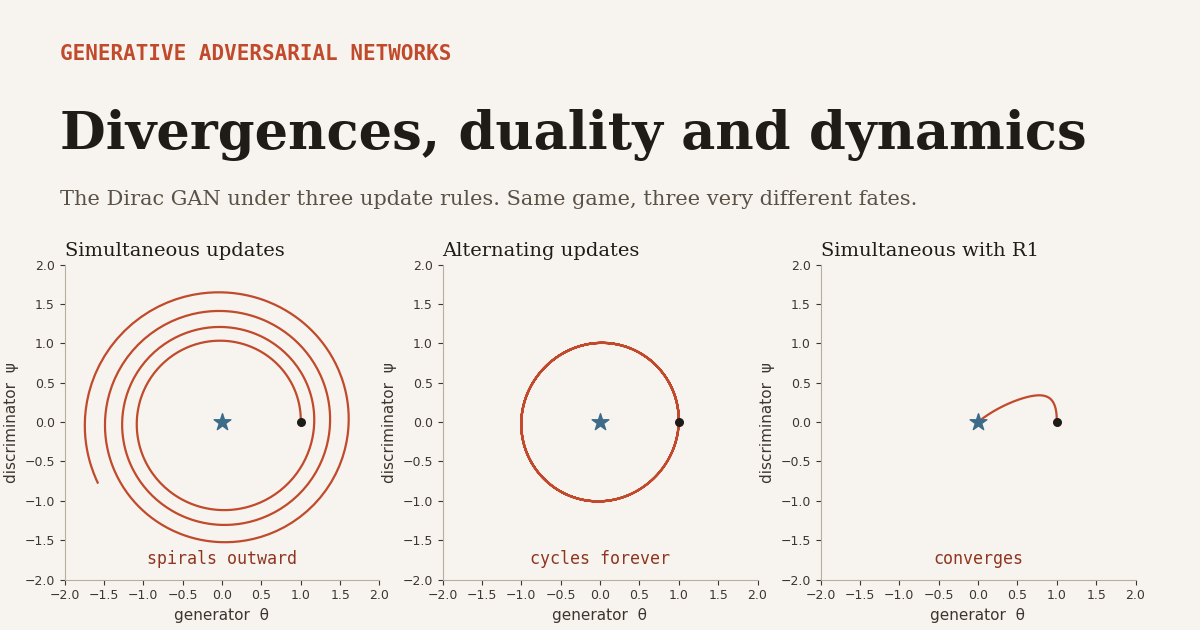
Lars Mescheder, Andreas Geiger and Sebastian Nowozin found the simplest example that exposes the problem, in Which Training Methods for GANs do actually Converge? at ICML 2018. They called it the Dirac GAN. Real data is a single point at 0. The generator outputs a single point at \( \theta \). The discriminator is linear, \( D_{\psi}(x) = \psi x \). With \( f(t) = -\log(1 + e^{-t}) \), the standard GAN objective becomes a function of two numbers.
The generator descends \( L \) and the discriminator ascends it, which gives the update direction \( v \). The only equilibrium is \( \theta = \psi = 0 \), the generator sitting on the data. Linearize around it. With \( f'(0) = 1/2 \), the Jacobian is a pure rotation.
Purely imaginary eigenvalues mean the continuous time dynamics circle the equilibrium forever. Discrete steps make it worse. A simultaneous gradient step of size \( h \) multiplies the state by \( I + hJ \), whose eigenvalues \( 1 \pm ih/2 \) have modulus \( \sqrt{1 + h^2/4} \), which is greater than 1. Every step pushes the state slightly further out. With \( h = 0.1 \), linear theory predicts growth by a factor of about 1.87 over 500 steps. The nonlinear simulation in the code starts at distance 1 from equilibrium and ends at 1.76, slightly less because \( f’ \) shrinks away from the origin. Alternating updates, where the discriminator sees the already updated generator, preserve area instead. Their trajectory stays on a closed orbit and ends at distance 0.99.
Here is the intuition. When the generator reaches the data, the discriminator’s slope \( \psi \) is at its largest, so the discriminator is still pushing the generator. The generator overshoots, the discriminator’s slope flips, and the pair chases each other around the target without ever settling.
The fix is to damp the discriminator. Mescheder and colleagues proposed a zero centred gradient penalty on real data.
For the Dirac GAN the input gradient is just \( \psi \), so the penalty adds \( -\gamma\psi \) to the discriminator’s update and the Jacobian gains a \( -\gamma \) in its lower right entry. Its eigenvalues become \( \big(-\gamma \pm \sqrt{\gamma^2 – 4f'(0)^2}\big)/2 \), which have negative real part for any \( \gamma > 0 \). With \( \gamma = 1 \) both eigenvalues equal \( -1/2 \), and the simulation converges to the origin. Their Theorem 4.1 extends local convergence with this penalty to realistic settings where both distributions lie on lower dimensional manifolds. The penalty’s zero centre matters. The WGAN-GP penalty pulls gradient norms toward 1, which does not vanish at equilibrium and does not give the same guarantee.
A related idea from Martin Heusel and colleagues, the two time scale update rule, gives the players different learning rates. Their TTUR paper proved convergence to a local Nash equilibrium under stochastic approximation assumptions when the discriminator learns on a faster time scale. It is also the paper that introduced FID.
A GAN has no single loss to go down. It has a vector field, and whether training converges depends on the eigenvalues of that field’s Jacobian at equilibrium. Rotation dominated Jacobians produce cycles and outward spirals. Zero centred gradient penalties add the damping that turns rotation into convergence.
Conditioning, the Projection Discriminator
Conditional GANs, introduced by Mehdi Mirza and Simon Osindero in Conditional Generative Adversarial Nets in 2014, generate a sample for a given label. Early versions simply concatenated the label to the discriminator’s input. Takeru Miyato and Masanori Koyama derived a better design from the optimal discriminator in cGANs with Projection Discriminator at ICLR 2018.
With a logistic output, the optimal conditional discriminator’s logit is the log density ratio, and Bayes’ rule splits it into two pieces.
Assume each conditional is a softmax over a shared feature \( \phi(x) \), so \( p(y = c \mid x) \propto \exp(v_c^{\top}\phi(x)) \). The label part becomes \( (v^{\text{data}}_y – v^{g}_y)^{\top}\phi(x) \) minus a difference of log normalizers that depends only on \( x \). Absorb every term that depends only on \( x \) into a single function \( \psi \) and write the label as a one hot vector \( y \).
The label enters through an inner product with the image features, a projection, rather than through concatenation at the input. That structure came straight from the algebra, and it became the standard way to condition large class conditional GANs.
Measuring What a GAN Learned
A GAN gives you a sampler and no likelihood, so evaluation needs its own mathematics. Tim Salimans and colleagues proposed the Inception Score in Improved Techniques for Training GANs in 2016.
It is high when each image is classified confidently, so \( p(y \mid x) \) is peaked, and when the classes across all images are varied, so the marginal \( p(y) \) is flat. It never looks at real data, which is its main weakness. A generator that produces one perfect image per class scores well while ignoring all variation within classes.
Heusel and colleagues fixed this with the Fréchet Inception Distance. Pass real and generated images through an Inception network, fit a Gaussian to each set of 2048 dimensional pool features, and compute the Fréchet distance between the two Gaussians.
This is exactly the squared Wasserstein 2 distance between two Gaussians, which ties evaluation back to the transport ideas of the Wasserstein GAN. The mean term catches samples that are off target. The trace term catches samples with the wrong spread, including the missing variety of mode collapse. The code checks the formula against the closed form for diagonal covariances.
FID has caveats worth stating. It assumes the features are Gaussian, which they are not. Its value depends on the number of samples used, so scores computed with different sample counts should not be compared. And it inherits whatever the Inception network happens to find important, which may not match what a human or a downstream task cares about.
What a Toy Experiment Shows
The code trains both a non saturating GAN and a WGAN-GP on a ring of eight tight Gaussian clusters, a standard test for mode collapse, using the same small networks and 2000 generator steps. It counts how many clusters receive at least 1 percent of samples and what fraction of samples land within 0.25 of a cluster centre.
| Loss | Seed 0 | Seed 1 | Seed 2 |
|---|---|---|---|
| Non saturating GAN, modes covered | 8 of 8 | 5 of 8 | 8 of 8 |
| Non saturating GAN, samples near a centre | 0.92 | 0.83 | 0.92 |
| WGAN-GP, modes covered | 8 of 8 | 8 of 8 | 8 of 8 |
| WGAN-GP, samples near a centre | 0.40 | 0.44 | 0.56 |
A single CPU run of the code below by aitrendblend. A toy illustration, not a benchmark.
The pattern is consistent with the theory. The non saturating GAN produced sharper samples but dropped three modes on one seed, the kind of behaviour Equation 5 leads you to expect. WGAN-GP covered every mode on every seed but placed fewer samples tightly on the clusters, which is consistent with a transport based loss that rewards moving mass roughly into place before sharpening it. Three seeds on a toy problem prove nothing on their own. They do show why practitioners describe the two losses as trading sharpness for coverage.
Reported Benchmark Numbers
The spectral normalization paper compared ways of controlling the discriminator under one standard convolutional architecture on CIFAR-10. Higher Inception Score is better and lower FID is better.
| Discriminator control | Inception Score | FID |
|---|---|---|
| Real data | 11.24 ± 0.12 | 7.8 |
| Weight clipping | 6.41 ± 0.11 | 42.6 |
| WGAN-GP | 6.68 ± 0.06 | 40.2 |
| Weight normalization | 6.84 ± 0.07 | 34.7 |
| Layer normalization | 7.19 ± 0.12 | 33.9 |
| Spectral normalization | 7.42 ± 0.08 | 29.3 |
Unsupervised CIFAR-10 with the standard CNN, as reported by Miyato et al. (2018), arXiv:1802.05957. Gulrajani et al. (2017) separately reported an Inception Score of 7.86 ± 0.07 for WGAN-GP with a ResNet architecture.
Two readings matter. Weight clipping, the crudest Lipschitz control, is worst on both metrics, as the theory suggests. And the architecture changes the picture, since WGAN-GP with a ResNet scores a higher Inception Score than every generated result in this table. Comparisons between loss functions are only meaningful with the architecture held fixed.
A Practical Recipe Grounded in the Math
Use the non saturating loss or a hinge loss, never the raw minimax loss, because Equation 4 shows the minimax version starves the generator early on. Accept that the non saturating loss leans toward mode dropping, and watch diversity explicitly rather than only watching sample quality.
Control the discriminator’s smoothness. Spectral normalization is the cheapest default and applies to any loss. Add an R1 penalty on real data when training is unstable, starting with a small \( \gamma \), because the Dirac GAN analysis shows it supplies exactly the damping that plain gradient steps lack. If you use a Wasserstein loss, prefer a gradient penalty to weight clipping.
Treat learning rates as a game design choice. Adam with a low first moment coefficient, around 0.5 or 0, and separate learning rates for the two players follow directly from the rotation dominated dynamics of Equation 13. Averaging the generator’s weights over time is another standard tool that smooths out the cycling.
Evaluate with FID computed on a fixed and reported number of samples, and pair it with a diversity or recall style metric when mode coverage matters. When a run collapses, the divergence view gives a checklist. Is the discriminator too sharp, is the loss mode seeking, and do the supports overlap at all?
Limitations and Open Questions
Most of the clean results in this article are local or idealized. The optimal discriminator derivation assumes unlimited capacity. The Dirac GAN convergence proofs are local, describing behaviour near an equilibrium that training may never approach. Global convergence of realistic GAN training remains unproven.
The divergence story is also incomplete. Sanjeev Arora and colleagues argued in Generalization and Equilibrium in Generative Adversarial Nets at ICML 2017 that with a finite discriminator the objective does not truly measure a divergence between full distributions, so a generator can score well against every discriminator in its class while still missing much of the data. Which distance a real, finite GAN minimizes is a subtler question than the tidy table in the f-GAN section suggests.
Gradient penalties have their own ambiguities. The WGAN-GP penalty is enforced on interpolated points chosen for convenience rather than on the transport lines its justification refers to, and the critic’s dual estimate is biased when the penalty is soft, as the 2.17 versus 2 result in the code shows.
Evaluation remains the weakest link. The Inception Score ignores real data, FID assumes Gaussian features and depends on sample size, and both rely on an ImageNet classifier whose notion of similarity may be irrelevant for medical, scientific or non photographic data.
Finally, diffusion models have overtaken GANs on many image benchmarks, partly because their training objective is a stable regression rather than a game. GANs keep a real advantage in speed, since they generate in one forward pass, and adversarial losses have been folded into faster diffusion samplers. Preference alignment has followed a similar path, as our review of DPO and RLHF for diffusion models shows. The realism these models reach has also created a detection problem, covered in our piece on vision transformers for face forgery detection. The mathematics of this article remains relevant precisely because the adversarial idea keeps being reused inside other systems.
Conclusion
The original GAN paper proved a clean theorem. With an optimal discriminator, the generator minimizes a Jensen Shannon divergence and succeeds exactly when it matches the data. Almost every practical difficulty since then traces back to the ways real training departs from that theorem, and each departure has a precise mathematical form.
The conceptual shift is to stop thinking of a GAN loss as a classifier’s error and to think of it as a choice of divergence, estimated by a critic and optimized through a game. Seen that way, saturation is a property of a logarithm, mode collapse is a property of reverse KL, vanishing gradients are a property of divergences that compare densities on non overlapping supports, and non convergence is a property of rotating eigenvalues.
The same ideas travel well. The Fenchel dual bound behind f-GANs reappears in mutual information estimation. Kantorovich duality underlies optimal transport methods across machine learning. Spectral normalization is used far beyond GANs to control the smoothness of any network, and zero centred gradient penalties are now standard in adversarial components of other generative models.
The open problems are real. Global convergence remains unproven, finite discriminators blur the divergence interpretation, and evaluation still leans on imperfect proxies. None of that makes the mathematics less useful. It makes it the most reliable guide available when a run starts to fail.
If you remember one derivation, make it Equation 4 and its consequence, Equation 5. The loss that made GANs trainable is also the loss that makes them drop modes. Most of the story that followed is an attempt to keep the first property and remove the second.
Complete PyTorch Implementation
The file below is an independent educational reimplementation written by aitrendblend, not official code from any of the papers cited. It checks the optimal discriminator identity by numerical integration, measures generator gradient saturation, verifies five f-GAN variational bounds, implements the WGAN-GP and R1 penalties and spectral normalization by power iteration, simulates the Dirac GAN under three update rules, computes the Fréchet distance used by FID, and trains a non saturating GAN and a WGAN-GP on an eight mode ring with a mode coverage metric. On a CPU it finishes in a few minutes.
"""
GAN mathematics in runnable form. Divergences, duality and training dynamics.
Independent educational implementation by aitrendblend. Not official code from any paper.

Contents
  1. Closed form densities and quadrature helpers for one dimensional checks
  2. The optimal discriminator and the Jensen Shannon identity
  3. Generator loss saturation, minimax versus non saturating
  4. f-GAN variational bounds with Fenchel conjugates
  5. Wasserstein critics, gradient penalty, R1 penalty and spectral normalization
  6. The Dirac GAN, simultaneous versus alternating updates versus R1
  7. Frechet distance between Gaussians (the formula behind FID)
  8. A full training loop on an eight mode ring, NS-GAN versus WGAN-GP, with a mode coverage metric
"""
import math
import torch
import torch.nn as nn
import torch.nn.functional as F

torch.manual_seed(0)
LOG2 = math.log(2.0)


# ---------------------------------------------------------------------------
# 1. Quadrature helpers
# ---------------------------------------------------------------------------
GRID = torch.linspace(-12, 12, 200001, dtype=torch.float64)
DX = float(GRID[1] - GRID[0])


def gauss(x, mu, s):
    return torch.exp(-0.5 * ((x - mu) / s) ** 2) / (s * math.sqrt(2 * math.pi))


def integrate(y):
    return float(torch.trapezoid(y, dx=DX))


def kl(p, q, eps=1e-300):
    m = p > 1e-30
    return integrate(torch.where(m, p * (torch.log(p + eps) - torch.log(q + eps)), torch.zeros_like(p)))


def jsd(p, q):
    m = 0.5 * (p + q)
    return 0.5 * kl(p, m) + 0.5 * kl(q, m)


# ---------------------------------------------------------------------------
# 2. Optimal discriminator
# ---------------------------------------------------------------------------
def optimal_discriminator(p_data, p_g):
    """D*(x) = p_data(x) / (p_data(x) + p_g(x))"""
    return p_data / (p_data + p_g)


def value_function(D, p_data, p_g, eps=1e-300):
    """V(D, G) = E_data log D + E_g log(1 - D)"""
    return integrate(p_data * torch.log(D + eps) + p_g * torch.log(1 - D + eps))


def check_optimal_discriminator_identity():
    """V(D*, G) = -log 4 + 2 JSD(p_data || p_g)."""
    p, q = gauss(GRID, 0.0, 1.0), gauss(GRID, 1.5, 0.7)
    lhs = value_function(optimal_discriminator(p, q), p, q)
    rhs = -math.log(4) + 2 * jsd(p, q)
    return abs(lhs - rhs) < 1e-6


def check_learned_discriminator_matches_optimum(steps=3000):
    """A small MLP trained with binary cross entropy converges toward D* = p / (p + q)."""
    torch.manual_seed(1)
    D = nn.Sequential(nn.Linear(1, 64), nn.Tanh(), nn.Linear(64, 64), nn.Tanh(), nn.Linear(64, 1))
    opt = torch.optim.Adam(D.parameters(), lr=3e-3)
    for _ in range(steps):
        xr = torch.randn(512, 1)
        xf = 1.5 + 0.7 * torch.randn(512, 1)
        loss = F.binary_cross_entropy_with_logits(D(xr), torch.ones(512, 1)) + \
               F.binary_cross_entropy_with_logits(D(xf), torch.zeros(512, 1))
        opt.zero_grad(); loss.backward(); opt.step()
    x = torch.linspace(-1.5, 3.0, 50, dtype=torch.float64)
    target = optimal_discriminator(gauss(x, 0, 1), gauss(x, 1.5, 0.7))
    with torch.no_grad():
        learned = torch.sigmoid(D(x.float()[:, None])).squeeze().double()
    return float((learned - target).abs().max())


# ---------------------------------------------------------------------------
# 3. Saturation
# ---------------------------------------------------------------------------
def generator_gradients(logit):
    """Gradient of each generator loss with respect to the discriminator logit on a fake sample."""
    l = torch.tensor(float(logit), requires_grad=True)
    minimax = torch.log(1 - torch.sigmoid(l))            # generator minimizes this
    minimax.backward()
    g_mm = float(l.grad)
    l.grad = None
    ns = -F.logsigmoid(l)                                # non saturating, generator minimizes -log D
    ns.backward()
    return g_mm, float(l.grad)


# ---------------------------------------------------------------------------
# 4. f-GAN
# ---------------------------------------------------------------------------
F_DIVERGENCES = {
    #  name          f(u)                                              f'(u)                                         f*(t)                                   output activation g_f(v)
    "kl":         (lambda u: u * torch.log(u),                         lambda u: 1 + torch.log(u),                   lambda t: torch.exp(t - 1),             lambda v: v),
    "reverse_kl": (lambda u: -torch.log(u),                            lambda u: -1 / u,                             lambda t: -1 - torch.log(-t),           lambda v: -torch.exp(-v)),
    "pearson":    (lambda u: (u - 1) ** 2,                             lambda u: 2 * (u - 1),                        lambda t: t ** 2 / 4 + t,               lambda v: v),
    "js":         (lambda u: -(u + 1) * torch.log((1 + u) / 2) + u * torch.log(u),
                   lambda u: torch.log(2 * u / (1 + u)),                 lambda t: -torch.log(2 - torch.exp(t)), lambda v: LOG2 - F.softplus(-v)),
    "gan":        (lambda u: u * torch.log(u) - (u + 1) * torch.log(u + 1),
                   lambda u: torch.log(u / (u + 1)),                     lambda t: -torch.log(1 - torch.exp(t)), lambda v: -F.softplus(-v)),
}


def f_divergence(name, p, q):
    f = F_DIVERGENCES[name][0]
    return integrate(q * f(p / q))


def variational_bound(name, T, p, q):
    """E_P[T] - E_Q[f*(T)], a lower bound on D_f(P || Q) for every T in the domain of f*."""
    fstar = F_DIVERGENCES[name][2]
    return integrate(p * T) - integrate(q * fstar(T))


def check_fenchel_bounds():
    """The bound is tight at T* = f'(p/q) and strictly smaller for a perturbed T."""
    p, q = gauss(GRID, 0.0, 1.0), gauss(GRID, 0.8, 1.2)
    mask = (GRID > -6) & (GRID < 6)
    p, q = p[mask], q[mask]
    ok = True
    for name, (f, fprime, fstar, act) in F_DIVERGENCES.items():
        exact = integrate(q * f(p / q))
        t_star = fprime(p / q)
        tight = variational_bound(name, t_star, p, q)
        loose = variational_bound(name, t_star * 0.9 if name != "reverse_kl" else t_star * 1.1, p, q)
        ok &= abs(exact - tight) < 1e-6 and loose < tight
    return ok


def check_gan_f_is_jsd():
    """With f(u) = u log u - (u + 1) log(u + 1), D_f = 2 JSD - log 4."""
    p, q = gauss(GRID, 0.0, 1.0), gauss(GRID, 2.0, 0.5)
    mask = (GRID > -7) & (GRID < 7)
    p, q = p[mask], q[mask]
    return abs(f_divergence("gan", p, q) - (2 * jsd(p, q) - math.log(4))) < 1e-5


def fgan_losses(name, v_real, v_fake):
    """Critic and generator losses for an f-GAN, given raw critic outputs v."""
    _, _, fstar, act = F_DIVERGENCES[name]
    t_real, t_fake = act(v_real), act(v_fake)
    critic_loss = -(t_real.mean() - fstar(t_fake).mean())      # critic maximizes the bound
    gen_loss = -fstar(t_fake).mean()                            # generator minimizes the bound, only E_Q[-f*(T)] depends on it
    return critic_loss, gen_loss


# ---------------------------------------------------------------------------
# 5. Lipschitz control
# ---------------------------------------------------------------------------
def gradient_penalty(critic, real, fake, lam=10.0):
    """WGAN-GP. lam * E[(||grad D(x_hat)|| - 1)^2], x_hat uniform on segments between real and fake."""
    eps = torch.rand(real.size(0), *[1] * (real.dim() - 1), device=real.device)
    x_hat = (eps * real + (1 - eps) * fake).requires_grad_(True)
    grad, = torch.autograd.grad(critic(x_hat).sum(), x_hat, create_graph=True)
    return lam * ((grad.flatten(1).norm(dim=1) - 1) ** 2).mean()


def r1_penalty(critic, real, gamma=10.0):
    """Mescheder et al. R1 = gamma / 2 * E_data ||grad D(x)||^2. Zero centred, on real data only."""
    real = real.detach().requires_grad_(True)
    grad, = torch.autograd.grad(critic(real).sum(), real, create_graph=True)
    return 0.5 * gamma * grad.flatten(1).pow(2).sum(1).mean()


def spectral_norm_power_iteration(W, iters=2000):
    """sigma(W) via v <- W^T u / ||W^T u||, u <- W v / ||W v||, sigma = u^T W v."""
    u = torch.randn(W.size(0), dtype=W.dtype)
    for _ in range(iters):
        v = F.normalize(W.T @ u, dim=0)
        u = F.normalize(W @ v, dim=0)
    return float(u @ W @ v)


def check_spectral_norm():
    W = torch.randn(64, 32, dtype=torch.float64)
    return abs(spectral_norm_power_iteration(W) - float(torch.linalg.matrix_norm(W, ord=2))) < 1e-6


def check_lipschitz_product_bound():
    """The Lipschitz constant of a ReLU network is at most the product of layer spectral norms."""
    torch.manual_seed(3)
    net = nn.Sequential(nn.Linear(8, 32), nn.ReLU(), nn.Linear(32, 32), nn.ReLU(), nn.Linear(32, 1)).double()
    bound = 1.0
    for m in net:
        if isinstance(m, nn.Linear):
            bound *= float(torch.linalg.matrix_norm(m.weight.detach(), ord=2))
    x = torch.randn(2000, 8, dtype=torch.float64, requires_grad=True)
    g, = torch.autograd.grad(net(x).sum(), x)
    return float(g.norm(dim=1).max()) <= bound + 1e-9


def w1_parallel_lines(theta):
    """Arjovsky et al. example. P0 = (0, Z), P_theta = (theta, Z), Z uniform. W1 = |theta|, JSD = log 2 for theta != 0."""
    return abs(theta), (0.0 if theta == 0 else LOG2), (0.0 if theta == 0 else float("inf"))


def estimate_w1_with_critic(theta=2.0, steps=1500):
    """Train a gradient penalized critic between the two parallel lines. Its dual value approaches |theta|."""
    torch.manual_seed(4)
    critic = nn.Sequential(nn.Linear(2, 64), nn.ReLU(), nn.Linear(64, 64), nn.ReLU(), nn.Linear(64, 1))
    opt = torch.optim.Adam(critic.parameters(), lr=1e-3, betas=(0.5, 0.9))
    for _ in range(steps):
        z = torch.rand(256, 1)
        real = torch.cat([torch.zeros_like(z), z], 1)
        fake = torch.cat([torch.full_like(z, theta), torch.rand(256, 1)], 1)
        loss = critic(fake).mean() - critic(real).mean() + gradient_penalty(critic, real, fake)
        opt.zero_grad(); loss.backward(); opt.step()
    with torch.no_grad():
        z = torch.rand(20000, 1)
        real = torch.cat([torch.zeros_like(z), z], 1)
        fake = torch.cat([torch.full_like(z, theta), torch.rand(20000, 1)], 1)
        return float(critic(real).mean() - critic(fake).mean())


# ---------------------------------------------------------------------------
# 6. Dirac GAN
# ---------------------------------------------------------------------------
def dirac_gan(mode="simultaneous", h=0.1, steps=500, gamma=0.0, theta0=1.0, psi0=0.0):
    """Generator delta_theta, discriminator D(x) = psi x, data delta_0, L = f(psi theta) + f(0),
    with f(t) = -log(1 + exp(-t)). Generator descends L, discriminator ascends L minus R1."""
    fprime = lambda t: torch.sigmoid(-torch.tensor(t)).item()     # f'(t) = 1 / (1 + e^t)
    theta, psi = theta0, psi0
    for _ in range(steps):
        g_theta = psi * fprime(theta * psi)
        if mode == "simultaneous":
            g_psi = theta * fprime(theta * psi) - gamma * psi
            theta, psi = theta - h * g_theta, psi + h * g_psi
        else:                                                        # alternating
            theta = theta - h * g_theta
            psi = psi + h * (theta * fprime(theta * psi) - gamma * psi)
    return math.hypot(theta, psi)


def dirac_jacobian_eigenvalues(gamma=0.0):
    """At the equilibrium the Jacobian is [[0, -f'(0)], [f'(0), -gamma]] with f'(0) = 1/2."""
    J = torch.tensor([[0.0, -0.5], [0.5, -gamma]], dtype=torch.float64)
    return torch.linalg.eigvals(J)


# ---------------------------------------------------------------------------
# 7. Frechet distance
# ---------------------------------------------------------------------------
def sqrtm_psd(M):
    evals, evecs = torch.linalg.eigh(M)
    return evecs @ torch.diag(evals.clamp_min(0).sqrt()) @ evecs.T


def frechet_distance(mu1, S1, mu2, S2):
    """||mu1 - mu2||^2 + Tr(S1 + S2 - 2 (S1^{1/2} S2 S1^{1/2})^{1/2}), the Gaussian W2 squared."""
    s1h = sqrtm_psd(S1)
    cross = sqrtm_psd(s1h @ S2 @ s1h)
    return float(((mu1 - mu2) ** 2).sum() + torch.trace(S1 + S2 - 2 * cross))


def check_frechet():
    d = 5
    mu1, mu2 = torch.zeros(d, dtype=torch.float64), torch.ones(d, dtype=torch.float64)
    s1, s2 = torch.full((d,), 1.0, dtype=torch.float64), torch.full((d,), 4.0, dtype=torch.float64)
    closed = float(((mu1 - mu2) ** 2).sum() + ((s1.sqrt() - s2.sqrt()) ** 2).sum())
    same = frechet_distance(mu1, torch.diag(s1), mu1, torch.diag(s1))
    return abs(frechet_distance(mu1, torch.diag(s1), mu2, torch.diag(s2)) - closed) < 1e-9 and abs(same) < 1e-9


# ---------------------------------------------------------------------------
# 8. Eight mode ring, a complete training loop
# ---------------------------------------------------------------------------
def ring_sampler(n, modes=8, radius=2.0, std=0.05):
    k = torch.randint(0, modes, (n,))
    ang = 2 * math.pi * k.float() / modes
    centers = torch.stack([radius * torch.cos(ang), radius * torch.sin(ang)], 1)
    return centers + std * torch.randn(n, 2)


def mlp(d_in, d_out, width=128):
    return nn.Sequential(nn.Linear(d_in, width), nn.ReLU(), nn.Linear(width, width), nn.ReLU(),
                         nn.Linear(width, width), nn.ReLU(), nn.Linear(width, d_out))


@torch.no_grad()
def mode_coverage(G, n=4000, modes=8, radius=2.0, tol=0.25, z_dim=2):
    """Modes that receive at least 1 percent of samples within tol, and the fraction of high quality samples."""
    x = G(torch.randn(n, z_dim))
    ang = 2 * math.pi * torch.arange(modes).float() / modes
    centers = torch.stack([radius * torch.cos(ang), radius * torch.sin(ang)], 1)
    d = torch.cdist(x, centers)
    nearest, idx = d.min(1)
    good = nearest < tol
    counts = torch.bincount(idx[good], minlength=modes)
    return int((counts > 0.01 * n).sum()), float(good.float().mean())


def train_gan(loss="ns", steps=2000, z_dim=2, batch=256, seed=0, lr=None):
    """Non saturating GAN (one D step per G step) or WGAN-GP (five critic steps per G step)."""
    torch.manual_seed(seed)
    G, D = mlp(z_dim, 2), mlp(2, 1)
    lr = lr or (5e-4 if loss == "ns" else 1e-4)
    betas = (0.5, 0.9)
    opt_g = torch.optim.Adam(G.parameters(), lr=lr, betas=betas)
    opt_d = torch.optim.Adam(D.parameters(), lr=lr, betas=betas)
    n_critic = 5 if loss == "wgan-gp" else 1
    for _ in range(steps):
        for _ in range(n_critic):
            real = ring_sampler(batch)
            fake = G(torch.randn(batch, z_dim)).detach()
            if loss == "ns":
                d_loss = F.softplus(-D(real)).mean() + F.softplus(D(fake)).mean()
            else:
                d_loss = D(fake).mean() - D(real).mean() + gradient_penalty(D, real, fake)
            opt_d.zero_grad(); d_loss.backward(); opt_d.step()
        fake = G(torch.randn(batch, z_dim))
        g_loss = F.softplus(-D(fake)).mean() if loss == "ns" else -D(fake).mean()
        opt_g.zero_grad(); g_loss.backward(); opt_g.step()
    return mode_coverage(G, z_dim=z_dim)


if __name__ == "__main__":
    print("V(D*,G) = -log4 + 2 JSD     ", check_optimal_discriminator_identity())
    print("learned D vs D*, max error  ", round(check_learned_discriminator_matches_optimum(), 3))
    for logit in [0.0, -2.0, -4.6]:
        mm, ns = generator_gradients(logit)
        print(f"logit {logit:5.1f}  D = {torch.sigmoid(torch.tensor(logit)).item():.3f}  "
              f"minimax grad {mm:+.3f}  non saturating grad {ns:+.3f}")
    print("Fenchel bounds tight at T*  ", check_fenchel_bounds())
    print("GAN f equals 2 JSD - log 4  ", check_gan_f_is_jsd())
    print("power iteration = sigma(W)  ", check_spectral_norm())
    print("Lipschitz <= product bound  ", check_lipschitz_product_bound())
    print("Frechet distance formula    ", check_frechet())
    print("parallel lines theta=2      ", "W1, JSD, KL =", w1_parallel_lines(2.0))
    print("critic estimate of W1       ", round(estimate_w1_with_critic(2.0), 3))
    print("Dirac Jacobian eigenvalues  ", dirac_jacobian_eigenvalues(0.0).tolist(), "with R1:", dirac_jacobian_eigenvalues(1.0).tolist())
    print("Dirac radius, simultaneous  ", round(dirac_gan("simultaneous"), 3))
    print("Dirac radius, alternating   ", round(dirac_gan("alternating"), 3))
    print("Dirac radius, simult. + R1  ", round(dirac_gan("simultaneous", gamma=1.0), 4))
    for loss in ["ns", "wgan-gp"]:
        for seed in range(3):
            modes, quality = train_gan(loss, seed=seed)
            print(f"{loss:8s} seed {seed}  modes covered {modes}/8, samples within tolerance {quality:.2f}")
The eight mode experiment is the slowest part. Reduce the number of seeds or steps in the main block for a quicker run. Results vary with seed, which is part of the point.
Frequently Asked Questions
Why do GANs suffer from mode collapse?
The loss most GANs actually use, the non saturating generator loss, follows the gradient of a reverse KL divergence minus twice the Jensen Shannon divergence when the discriminator is optimal. Reverse KL heavily penalizes generated samples that look unrealistic but barely penalizes real modes the generator ignores, so a generator can lower its loss by producing convincing samples from only a few modes.
What divergence does the original GAN minimize?
With an optimal discriminator, the original minimax objective equals twice the Jensen Shannon divergence between the data and generator distributions minus log 4. Its minimum is reached exactly when the two distributions are equal. In practice the discriminator is never optimal and most implementations use the non saturating loss, which follows a different divergence.
Why does the Wasserstein GAN give better gradients?
When real and generated data lie on thin sets that do not overlap, divergences that compare densities point by point, such as KL and Jensen Shannon, become constant or infinite and provide no direction to improve. The Wasserstein distance measures how far probability mass must move, so it shrinks smoothly as the generator approaches the data even when the supports never touch.
What is the difference between WGAN-GP and the R1 penalty?
WGAN-GP penalizes the squared difference between the critic’s gradient norm and 1 at points interpolated between real and fake samples, which approximately enforces the Lipschitz constraint that the Wasserstein dual form needs. R1 penalizes the squared gradient norm itself on real data only, pulling it toward zero. The zero centred R1 penalty damps the rotating dynamics of the game and comes with local convergence guarantees.
How does spectral normalization stabilize a GAN?
It divides each weight matrix of the discriminator by its largest singular value, estimated cheaply with one step of power iteration per update. Because the Lipschitz constant of a layered network is at most the product of its layers’ spectral norms, this caps how sharply the discriminator can change, which keeps its gradients informative and prevents it from overpowering the generator.
Is FID a reliable way to compare GANs?
FID is the most widely used metric, but it has limits. It fits Gaussians to Inception network features even though those features are not Gaussian, its value depends on the number of samples used, and it reflects what an ImageNet classifier considers similar. Compare FID only with the same sample count and feature extractor, and pair it with a diversity measure when mode coverage matters.
Read the papers behind the math
Arjovsky and Bottou explain why GAN gradients vanish and why the non saturating loss drops modes. Mescheder, Geiger and Nowozin show why GAN training cycles and how R1 fixes it.
Primary citation. Goodfellow, I., Pouget-Abadie, J., Mirza, M., Xu, B., Warde-Farley, D., Ozair, S., Courville, A., and Bengio, Y. (2014). Generative Adversarial Nets. NeurIPS 2014. arXiv:1406.2661.
Also cited. Arjovsky and Bottou (ICLR 2017). Arjovsky, Chintala and Bottou (ICML 2017). Nowozin, Cseke and Tomioka (NeurIPS 2016). Mao et al. (ICCV 2017). Gulrajani et al. (NeurIPS 2017). Miyato et al. (ICLR 2018). Mescheder, Geiger and Nowozin (ICML 2018). Heusel et al. (NeurIPS 2017). Mirza and Osindero (2014). Miyato and Koyama (ICLR 2018). Salimans et al. (NeurIPS 2016). Arora et al. (ICML 2017).
This analysis is based on the published papers and an independent evaluation of their claims.