In 2014 Ian Goodfellow and his coauthors described a training setup that sounded almost like a prank. Take two neural networks, point them at each other, and let one try to fool the other forever. One network paints fake images. The other decides whether each image is real or painted. Neither is told what a good image looks like. They only get the verdict of the contest. Out of that single idea came a decade of photoreal faces, image translation, and a whole research field built on competition rather than imitation.
Key points
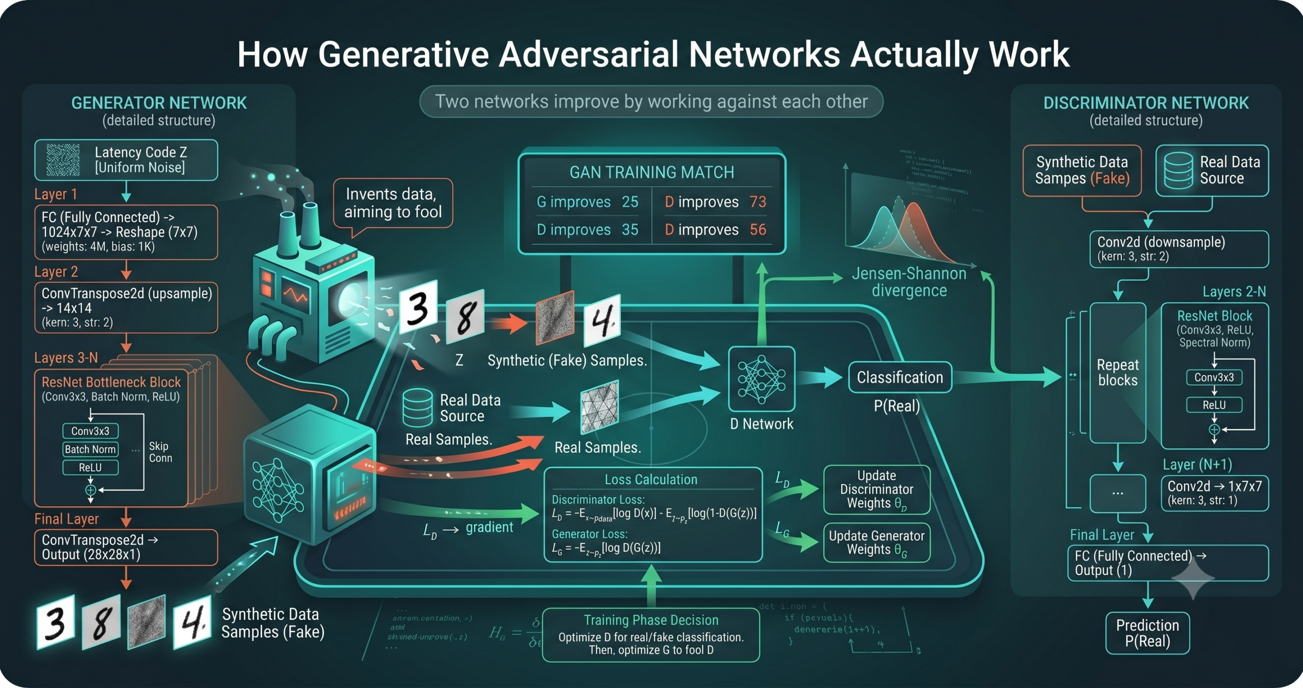
- A GAN trains two networks at once, a generator that maps random noise to fake samples and a discriminator that tries to separate fakes from real data.
- The training objective is a minimax game, and the original paper proves that the best possible discriminator turns the game into a measure of distance between the real and generated distributions.
- At the global optimum the generated distribution exactly matches the data distribution, which is the formal reason the method can work at all.
- In practice the game is hard to balance, and the famous failures are mode collapse and vanishing gradients for the generator.
- Later work such as DCGAN, Wasserstein GAN, and spectral normalization fixed much of the instability without changing the core adversarial idea.
- A complete and runnable PyTorch DCGAN is included at the end so you can watch the dynamics yourself.
The problem GANs were built to solve
Most of deep learning is about prediction. You hand the model an input and ask for a label, a number, or a translation. Generation flips that around. You want the model to produce brand new samples that look like they came from your training set, faces that no camera ever captured, molecules nobody has synthesized, audio of a voice saying something it never said.
The hard part is that we rarely have a clean formula for what real data looks like. The distribution of natural images lives in a space of millions of pixels, and almost every point in that space is noise. The tiny sliver that looks like a real photograph has no closed form. Classical approaches tried to write down a probability density and maximize its likelihood, which works beautifully for simple cases and becomes a nightmare for images, because the normalizing constant that makes a density sum to one is usually impossible to compute.
Researchers had known for years that you can sidestep that constant if you are willing to give up an explicit density and settle for a way to draw samples. Variational autoencoders, introduced by Kingma and Welling in arXiv:1312.6114, took one route through a learned latent space and a reconstruction objective. GANs took a stranger route. They never write down a density at all. They learn to sample by learning to fool a critic.
The adversarial idea in plain terms
Think of a counterfeiter and a bank inspector. The counterfeiter prints fake notes and wants them to pass. The inspector studies notes and tries to flag the fakes. Early on the counterfeiter is clumsy and the inspector catches everything. The counterfeiter learns from each rejection and prints something a little better. The inspector, now fooled more often, sharpens its eye. Round after round the fakes improve, because the only teacher the counterfeiter has is the inspector who keeps getting harder to beat.
That is the whole intuition. The generator is the counterfeiter, the discriminator is the inspector, and the training data is the supply of genuine notes. The clever part is that the generator never sees a real example directly. It only ever receives a gradient that says make the discriminator more uncertain. The realism is squeezed out of the contest itself. For a friendly tour of where this leads in applications, our earlier overview of the power of generative adversarial networks covers the downstream uses, while this piece stays on the mechanism.
The minimax game written down
Let the data come from a distribution we call p data. The generator takes a noise vector z drawn from a simple prior, often a standard normal, and maps it to a sample G of z. Write the generated distribution as p g. The discriminator D outputs a single number between zero and one, its estimate that an input is real. The two networks play the following game.
Read it slowly. The discriminator wants to push D of x toward one for real samples and D of G of z toward zero for fakes, which maximizes the expression. The generator wants the opposite, it wants the discriminator to call its fakes real, which minimizes the same expression. There is no separate target image, no pixelwise loss against a ground truth. The entire signal is the disagreement between the two players.
Why this game has a meaningful solution
The reason the setup is more than a cute analogy is a short proof in the original paper. Fix the generator for a moment and ask what the best possible discriminator would be. For any input x, the optimal discriminator balances the two distributions and takes a clean form.
Substitute that optimal critic back into the value function and the generator is no longer fighting an arbitrary network. It is now minimizing a precise quantity.
The term JSD is the Jensen Shannon divergence, a symmetric measure of how far apart two distributions are. It is zero only when the two match and positive otherwise. So when the discriminator is doing its job perfectly, the generator is literally being pushed to make its distribution equal to the real one. The global best the generator can reach is a value of minus log four, and it reaches it exactly when p g equals p data. That is the formal promise of the method. If both networks had unlimited capacity and training were perfect, the generator would recover the true data distribution.
The gap between the proof and reality
Here is where it gets interesting. That elegant guarantee assumes an optimal discriminator at every step and infinite capacity. Real training has neither. We update the discriminator a few steps, update the generator a few steps, and hope the dance stays balanced. It often does not.
The first practical problem shows up in the generator loss. The minus log of one minus D term saturates. Early in training the discriminator easily rejects the generator output, D of G of z sits near zero, and the gradient that should teach the generator is almost flat. The generator learns slowly exactly when it most needs to learn fast. Goodfellow and his coauthors noticed this immediately and proposed a fix in the same paper. Rather than minimizing the log of one minus D, the generator maximizes the log of D directly.
This non saturating version gives the generator a strong gradient when its samples are being rejected, which is the moment that matters most. Almost every working GAN since uses this form rather than the textbook minimax loss, even though the textbook version is the one that carries the clean theory.
Mode collapse, the failure everyone hits
The second problem is stranger and harder. A generator can discover that one very convincing output fools the current discriminator, and then it produces that output again and again. Picture a model trained on handwritten digits that learns to draw a single gorgeous three and nothing else. The discriminator eventually catches on and penalizes that three, the generator hops to a perfect eight, and the two chase each other around a few favorite samples without ever covering the full variety of the data. This is mode collapse, and it is the single most common reason a GAN looks like it is training while producing almost no diversity.
Mode collapse happens because the generator objective rewards fooling the critic right now, not covering every mode of the data. Nothing in the basic loss demands diversity. The generator is free to dump all of its probability mass on whatever the discriminator currently finds hardest to reject.
The generator is rewarded for fooling today’s discriminator, not for matching tomorrow’s full distribution. That mismatch is the seed of most GAN pathologies.A common reading of the GAN training problem
How the architecture grew up
The 2014 paper used simple multilayer perceptrons and showed results on small datasets. The leap to convincing images came a year later with the deep convolutional GAN from Radford, Metz, and Chintala in arXiv:1511.06434. They replaced the dense layers with strided convolutions, used batch normalization to keep activations healthy, dropped pooling in favor of learned downsampling, and settled on a set of architectural rules that made training far more reliable. The generator became a stack of transposed convolutions that grow a small noise vector into a full image, and the discriminator became an ordinary convolutional classifier with a single real or fake output.
The DCGAN recipe is still the sensible starting point for anyone building a GAN from scratch, which is why the implementation at the end of this article follows it closely. The same training dynamics that affect every deep network show up here too, and our note on how batch size changes what a network learns is worth keeping in mind when a GAN refuses to settle.
What the original results actually showed
The first paper did not have the evaluation tools we take for granted now. There was no Frechet Inception Distance yet. To put a number on quality the authors fit a Parzen window density to generated samples and reported a log likelihood estimate on held out data. The headline figures are below.
| Dataset | Model | Parzen window log likelihood |
|---|---|---|
| MNIST | Adversarial nets | 225 with a standard error near 2 |
| MNIST | Deep GSN (prior work) | 214 with a standard error near 1.1 |
| TFD | Adversarial nets | 2057 with a standard error near 26 |
Figure 1. Parzen window log likelihood estimates reported in Goodfellow et al., NeurIPS 2014. Higher is better. The authors flagged the metric as imperfect.
Treat those numbers with care, because the authors themselves did. A later study by Theis, van den Oord, and Bethge in arXiv:1511.01844 showed that Parzen window estimates can rank models in misleading ways, especially in high dimensions. The honest reading is that the 2014 results were a proof of feasibility rather than a proof of superiority. The visual samples, blurry by today’s standards but clearly digit shaped and face shaped, did most of the persuading.
The fixes that made GANs trustworthy
The instability of the early years drove a wave of work aimed squarely at the training problem. The Wasserstein GAN from Arjovsky, Chintala, and Bottou in arXiv:1701.07875 swapped the Jensen Shannon objective for the earth mover distance, which gives smoother gradients even when the two distributions barely overlap. We covered the deeper convergence theory for this family in our piece on Wasserstein convergence guarantees for score based generative models, and the same distance sits at the heart of the Wasserstein GAN.
The first Wasserstein GAN enforced its constraint by clipping weights, a blunt tool that Gulrajani and coauthors replaced with a gradient penalty in arXiv:1704.00028. Miyato and coauthors then introduced spectral normalization in arXiv:1802.05957, a lightweight way to control the discriminator that became a default in many later models. On the evaluation side, the Frechet Inception Distance from Heusel and coauthors in arXiv:1706.08500 finally gave the field a metric that tracks human judgment reasonably well, and the Inception Score from Salimans and coauthors in arXiv:1606.03498 came a little earlier with the same goal.
Where GANs sit today
Diffusion models have taken the spotlight for raw image quality and training stability, and for good reason. They optimize a stable regression objective and avoid the balancing act entirely. Yet GANs are far from retired. They generate in a single forward pass, which makes them dramatically faster at inference than a diffusion model that needs dozens or hundreds of denoising steps. That speed keeps them alive in real time settings, on device generation, super resolution, and as components inside larger systems. The competition framework also reappears in places that have nothing to do with images, from domain adaptation to privacy research.
Honest limitations
The limitations are not footnotes, they are the reason the field spent years on fixes. Training requires balancing two networks, and if the discriminator becomes too strong the generator gradient vanishes, while if it becomes too weak the generator has nothing to learn from. Mode collapse remains a real risk that no single trick fully removes. Evaluation is genuinely hard, and the original Parzen window numbers above are a reminder that an impressive metric can be an artifact of the metric rather than the model, a point made directly by Theis and coauthors. The theory that guarantees convergence assumes infinite capacity and an optimal discriminator at every step, neither of which holds in practice, so the clean global optimum is a guidepost rather than a promise. Finally, GANs give you a sampler and not a density, so you cannot ask a trained GAN for the probability of a given example, which rules them out of tasks that need explicit likelihoods.
Conclusion
The reason the GAN idea endured is that it reframed generation as a contest rather than an imitation. Instead of telling a model what a good sample looks like, it built an opponent whose only job is to find flaws, and let the search for realism emerge from that pressure. The short proof that the adversarial loss becomes a divergence between distributions is what separates this from a clever trick, because it shows the method is chasing the right target even when the training is messy.
The conceptual shift matters beyond images. Once you accept that you can learn a distribution by learning to fool a critic, the same pattern transfers to audio, to text representations, to simulation, and to settings where two objectives naturally oppose each other. The generator and discriminator are just one instance of a broader idea about learning through competition.
The practical story is a story of taming. The first version worked in theory and stumbled in practice. The deep convolutional recipe stabilized the architecture, the Wasserstein objective fixed the gradients, gradient penalties and spectral normalization tamed the discriminator, and better metrics let researchers tell real progress from wishful thinking. None of those advances threw out the original game. They made it survivable.
The remaining limitations are real and worth respecting. Balancing two networks is still delicate, mode collapse still lurks, and the absence of an explicit density still rules GANs out of some jobs. A practitioner who reaches for a GAN should do so because the single pass speed or the adversarial framing buys something specific, not out of habit.
The clearest way to understand any of this is to watch it happen. Run the DCGAN below on a small dataset, then deliberately make the discriminator too strong and watch the generator stall, or remove the non saturating loss and watch the early training crawl. The math predicts every one of those behaviors, and seeing them line up with the equations is the moment GANs stop feeling like magic.
Complete DCGAN implementation in PyTorch
The following is a full and runnable deep convolutional GAN. It includes the generator, the discriminator, the non saturating loss, a training loop, a sampling function, and a smoke test on dummy data so you can confirm the shapes and the training step work before pointing it at a real dataset.
# Minimal but complete DCGAN in PyTorch
# Generator maps a noise vector to a 64x64 image, discriminator scores real vs fake
import torch
import torch.nn as nn
from torch.utils.data import DataLoader, TensorDataset

# ---- Hyperparameters ----
Z_DIM     = 100     # length of the noise vector
G_FEAT    = 64      # base feature width for the generator
D_FEAT    = 64      # base feature width for the discriminator
IMG_CH    = 3       # image channels, 3 for color
LR        = 2e-4    # learning rate from the DCGAN paper
BETAS     = (0.5, 0.999)  # Adam betas, the 0.5 term stabilizes GAN training


class Generator(nn.Module):
    # Transposed convolutions grow a 1x1 noise map into a 64x64 image
    def __init__(self, z_dim=Z_DIM, g=G_FEAT, ch=IMG_CH):
        super().__init__()
        def block(i, o, k=4, s=2, p=1):
            return nn.Sequential(
                nn.ConvTranspose2d(i, o, k, s, p, bias=False),
                nn.BatchNorm2d(o),
                nn.ReLU(True),
            )
        self.net = nn.Sequential(
            block(z_dim, g * 8, k=4, s=1, p=0),  # 1x1 -> 4x4
            block(g * 8, g * 4),                # 4x4 -> 8x8
            block(g * 4, g * 2),                # 8x8 -> 16x16
            block(g * 2, g),                    # 16x16 -> 32x32
            nn.ConvTranspose2d(g, ch, 4, 2, 1),      # 32x32 -> 64x64
            nn.Tanh(),                          # output in [-1, 1]
        )

    def forward(self, z):
        return self.net(z)


class Discriminator(nn.Module):
    # A standard conv classifier that ends in a single logit
    def __init__(self, ch=IMG_CH, d=D_FEAT):
        super().__init__()
        def block(i, o, bn=True):
            layers = [nn.Conv2d(i, o, 4, 2, 1, bias=False)]
            if bn:
                layers.append(nn.BatchNorm2d(o))
            layers.append(nn.LeakyReLU(0.2, True))
            return nn.Sequential(*layers)
        self.net = nn.Sequential(
            block(ch, d, bn=False),  # 64x64 -> 32x32
            block(d, d * 2),         # 32x32 -> 16x16
            block(d * 2, d * 4),     # 16x16 -> 8x8
            block(d * 4, d * 8),     # 8x8 -> 4x4
            nn.Conv2d(d * 8, 1, 4, 1, 0),  # 4x4 -> 1x1 logit
        )

    def forward(self, x):
        return self.net(x).view(-1)  # flatten to a vector of logits


def weights_init(m):
    # DCGAN initializes weights from a normal with std 0.02
    if isinstance(m, (nn.Conv2d, nn.ConvTranspose2d, nn.BatchNorm2d)):
        nn.init.normal_(m.weight, 0.0, 0.02)


def train_step(G, D, real, opt_g, opt_d, bce, device):
    # One full update of the discriminator then the generator
    bs = real.size(0)
    real = real.to(device)
    real_label = torch.ones(bs, device=device)
    fake_label = torch.zeros(bs, device=device)

    # ---- Train discriminator, maximize log D(x) + log(1 - D(G(z))) ----
    opt_d.zero_grad()
    logits_real = D(real)
    loss_real = bce(logits_real, real_label)
    z = torch.randn(bs, Z_DIM, 1, 1, device=device)
    fake = G(z)
    logits_fake = D(fake.detach())          # detach so G is not updated here
    loss_fake = bce(logits_fake, fake_label)
    loss_d = loss_real + loss_fake
    loss_d.backward()
    opt_d.step()

    # ---- Train generator with the non saturating loss, maximize log D(G(z)) ----
    opt_g.zero_grad()
    logits = D(fake)                        # reuse the fake batch, gradients flow to G now
    loss_g = bce(logits, real_label)        # label fakes as real to flip the sign
    loss_g.backward()
    opt_g.step()
    return loss_d.item(), loss_g.item()


@torch.no_grad()
def sample(G, n, device):
    # Draw n images from the generator for inspection
    G.eval()
    z = torch.randn(n, Z_DIM, 1, 1, device=device)
    imgs = G(z)
    G.train()
    return imgs  # values in [-1, 1], rescale to [0, 1] for display


def smoke_test():
    # Confirm shapes and a training step on random data, no real dataset needed
    device = torch.device('cuda' if torch.cuda.is_available() else 'cpu')
    G = Generator().to(device).apply(weights_init)
    D = Discriminator().to(device).apply(weights_init)
    bce = nn.BCEWithLogitsLoss()
    opt_g = torch.optim.Adam(G.parameters(), lr=LR, betas=BETAS)
    opt_d = torch.optim.Adam(D.parameters(), lr=LR, betas=BETAS)

    # 256 fake RGB images at 64x64 standing in for a dataset
    data = torch.rand(256, IMG_CH, 64, 64) * 2 - 1
    loader = DataLoader(TensorDataset(data), batch_size=32, shuffle=True)

    for epoch in range(2):
        for (batch,) in loader:
            ld, lg = train_step(G, D, batch, opt_g, opt_d, bce, device)
        print(f'epoch {epoch}  loss_d {ld:.3f}  loss_g {lg:.3f}')

    out = sample(G, 8, device)
    assert out.shape == (8, IMG_CH, 64, 64), out.shape
    print('ok, generated batch shape', tuple(out.shape))


if __name__ == '__main__':
    smoke_test()
Read the paper that started it all, then try the code on a real dataset such as CelebA or CIFAR-10.
Read the GAN paper Get a datasetFrequently asked questions
What is a generative adversarial network in simple terms
A generative adversarial network trains two neural networks against each other. A generator creates fake samples from random noise, and a discriminator tries to tell the fakes apart from real data. As the discriminator improves, the generator is forced to make more convincing samples, and the two keep pushing each other to get better.
What is the difference between the generator and the discriminator
The generator turns a random noise vector into a sample such as an image, and it never sees real data directly. The discriminator receives both real and generated samples and outputs a score for how real each one looks. The generator learns only from the discriminator’s judgments, while the discriminator learns from labeled real and fake examples.
Why are GANs so hard to train
Training a GAN means balancing two networks that improve at the same time. If the discriminator gets too strong the generator receives almost no useful gradient and stops learning, and if it gets too weak the generator has nothing to push against. The most common failure is mode collapse, where the generator produces only a few outputs that happen to fool the current discriminator instead of covering the full variety of the data.
What is mode collapse
Mode collapse is when a generator learns to produce a small number of outputs again and again rather than the full range of the training data. It happens because the basic loss rewards fooling the current discriminator and never explicitly demands diversity, so the generator can place all of its effort on whatever the critic finds hardest to reject.
Are GANs still used now that diffusion models exist
Yes. Diffusion models often win on raw image quality and stable training, but they need many steps to generate a single sample. GANs generate in one forward pass, which makes them much faster at inference and keeps them useful for real time generation, super resolution, on device models, and as components inside larger systems.
What is the best way to start building a GAN
Start from the deep convolutional GAN recipe, which uses strided convolutions, batch normalization, and the non saturating generator loss. Train on a small well understood dataset first, watch the generator and discriminator losses, and only scale up once the basic dynamics are stable. The PyTorch implementation in this article is a working starting point.
Goodfellow, I., Pouget-Abadie, J., Mirza, M., Xu, B., Warde-Farley, D., Ozair, S., Courville, A., and Bengio, Y. Generative Adversarial Nets. Advances in Neural Information Processing Systems 2014. arXiv:1406.2661. Additional works referenced include Radford et al. arXiv:1511.06434, Arjovsky et al. arXiv:1701.07875, Gulrajani et al. arXiv:1704.00028, Miyato et al. arXiv:1802.05957, Heusel et al. arXiv:1706.08500, Salimans et al. arXiv:1606.03498, Theis et al. arXiv:1511.01844, and Kingma and Welling arXiv:1312.6114.
This analysis is based on the published paper and an independent evaluation of its claims.