Key Points
- Both full-batch gradient descent and mini-batch SGD find global minima on this task, so the difference is not about optimization quality.
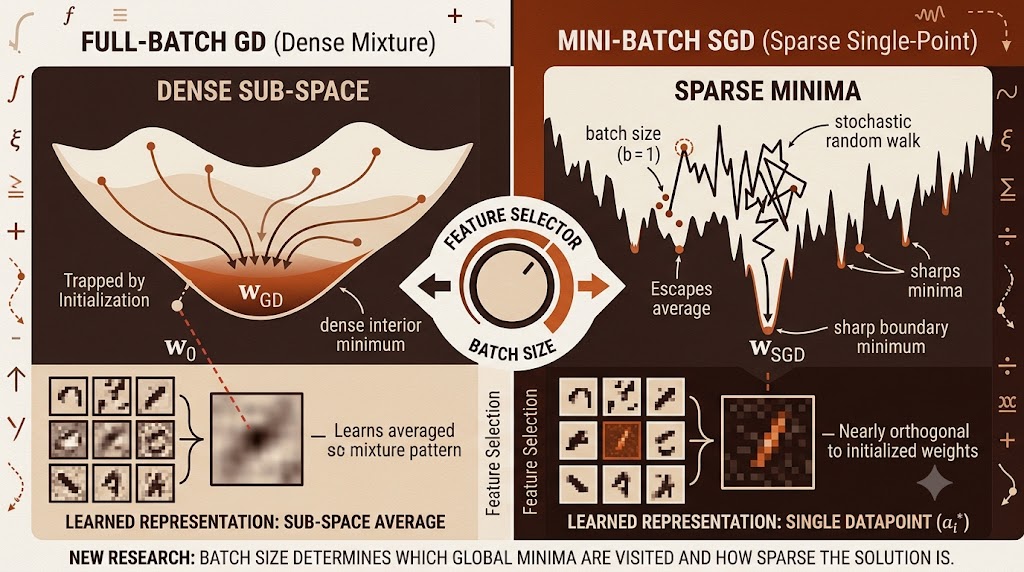
- Full-batch GD converges to a dense solution that mirrors the initialization direction and learns only a smeared average of the data.
- Any batch size strictly smaller than the full dataset drives SGD toward a single training datapoint — a sparse, data-dependent solution nearly orthogonal to where training started.
- Smaller batches produce sharper minima by the trace-of-Hessian measure, which contradicts one of the most-cited explanations for why large batches generalize poorly.
- The convergence proof for constant step size SGD uses tools from non-homogeneous random walk theory, a connection that may unlock new analysis techniques across machine learning.
- Cyclic SGD with a deterministic batch order shows the same sparse-convergence behavior, so true randomness is not the essential ingredient — small batch size is.
The Question Nobody Had Actually Answered
The idea that batch size shapes generalization dates back at least to Keskar et al. (2017), who showed empirically that large-batch training reliably finds sharper minima and those minima tend to generalize worse. The explanation became common wisdom: stochastic noise from small batches acts like an implicit regularizer, nudging the optimizer away from sharp ravines and toward flatter valleys.
What was never cleanly proved, though, is whether standard SGD — with a real mini-batch, real gradients, and a constant step size — actually converges to a qualitatively different solution than gradient descent on the full dataset. Most theoretical analysis sidesteps this by either adding explicit label noise, taking the step size to zero, or treating the noise as a surrogate continuous process. Nikhil Ghosh, Spencer Frei, Wooseok Ha, and Bin Yu decided to answer the question directly.
Their paper, published in JMLR in January 2025, studies a single-neuron weight-tied autoencoder trained on orthonormal data. The model is deliberately simple. That simplicity is the point — it is complex enough to be non-convex (there is a whole manifold of global minima) while being tractable enough that you can prove exactly where GD and SGD land.
The Setup
The autoencoder maps an input \( \mathbf{x} \) through a single neuron \( \mathbf{w} \), computes \( \phi(\langle \mathbf{w}, \mathbf{x} \rangle) \), and reconstructs the output as \( \mathbf{w} \phi(\langle \mathbf{w}, \mathbf{x} \rangle) \). The training set consists of \( m \) orthonormal vectors \( \mathbf{a}_1, \ldots, \mathbf{a}_m \in \mathbb{R}^n \), and the loss is the standard squared reconstruction error.
Orthonormal training data might sound like an unrealistic special case. The authors frame it as a simplified sparse coding model — one where the dictionary is orthogonal and each sample is a one-hot latent code. That framing matters for interpreting the results, but the math works for any orthonormal set.
With the activation \( \phi \) set to the identity, the reconstruction loss is
The global minima of this loss form a manifold. For the ReLU version they are all non-negative combinations of the training points whose squared coefficients sum to one. For the linear version the same manifold appears without the sign constraint. Any point on that manifold is equally good by the training objective — which is exactly what makes the choice between GD and SGD so interesting, because they end up at completely different corners of it.
What Full-Batch Gradient Descent Learns
The first theorem is both clean and a little unsettling. Under the conditions \( \|\mathbf{w}_0\| < 1 \) and step size \( \eta \leq 1/5 \), full-batch GD converges to
where \( \Pi_m \) is the orthogonal projection onto the span of the training data. The solution is the initialization projected onto the data subspace and then normalized. Nothing more.
Think about what that means in practice. If you randomly initialize \( \mathbf{w}_0 \) from a Gaussian, the projection picks up a small component of every training direction. The GD solution ends up as a roughly equal mixture of all \( m \) training vectors. It has learned the data subspace but not any particular feature within it. The paper calls this a “dense” solution, and the cosine similarity with any individual training point stays small — on the order of \( \sqrt{\log m / m} \) with high probability. The solution is not learning to recognize individual patterns; it is averaging them.
There is also a symmetry argument worth sitting with. Full-batch GD is invariant to orthogonal transformations that preserve the data span. You could rotate all the training points within their subspace and end up at the same solution. The model is responding to the geometry of the subspace, not to the identity of the training examples.
What Mini-Batch SGD Learns
The SGD result is the more surprising one. For any batch size strictly smaller than \( m \), the SGD iterates converge almost surely to a single training vector \( \mathbf{a}_{i^\star} \) (or its negative, depending on the sign of the initial correlation). Not a mixture. Not an average. One point.
The convergence set is
where \( \mathcal{S}^+ \) is the set of training directions that have positive initial correlation with the starting weights. The particular \( \mathbf{a}_{i^\star} \) selected is random — the theory does not pin down the probability distribution over the \( m \) candidates — but the qualitative fact is certain: you end up perfectly aligned with a single training point and nearly orthogonal to your random starting position.
The practical framing here is feature selection. The network is not averaging the training signals; it is choosing one and committing to it. In a sparse coding context this means SGD recovers an atom of the dictionary. In a more applied setting it suggests that small batch sizes genuinely change which features the network extracts, not just how quickly it converges.
“For random initializations, SGD learns a ‘pure’ datapoint whereas GD learns a ‘mixture’.”
Ghosh, Frei, Ha, and Yu — JMLR 2025Corollary 3 in the paper makes this quantitative. With high probability over a Gaussian initialization and both \( m \) and \( n \) large:
| Quantity | Full-Batch GD | Mini-Batch SGD |
|---|---|---|
| Max cosine similarity with training data | \( O\!\left(\sqrt{\log m / m}\right) \) — stays small | 1 — perfectly aligned with one point |
| Cosine similarity with initialization | \( \Theta(m/n) \) — stays close to start | \( O\!\left(\sqrt{\log m / n}\right) \) — nearly orthogonal |
| Solution type | Dense mixture of all training points | 1-sparse, exactly one training vector |
| Invariance to data rotations | Yes — only span matters | No — specific vector selected |
When \( n \) is large and \( m \) is on the same order, the GD solution barely moves from its starting point in the feature space, while the SGD solution ends up somewhere almost perpendicular to it. The network is not just following gradients differently — it is operating in a genuinely different learning regime.
Does Randomness Actually Matter?
This is an interesting question the paper takes care to address. Is the sparse-convergence behavior of SGD really about the randomness of the mini-batches, or just about their size?
Theorem 4 studies cyclic SGD — a completely deterministic variant where the batch at each step is just \( \{t \bmod m\} \), cycling through the training points in order. In the two-dimensional case with \( m = n = 2 \), cyclic SGD starting from the region where \( \langle \mathbf{w}_0, \mathbf{a}_0 \rangle \geq \langle \mathbf{w}_0, \mathbf{a}_1 \rangle > 0 \) converges to \( \mathbf{a}_0 \) almost surely.
The explicit limit is pinned down here unlike in the random case, and there is an interpretable intuition: the updates are biased toward whichever training vector currently has the highest correlation with the weights. The system drifts toward that point and eventually locks in. No randomness required.
The authors conjecture this holds for arbitrary \( m \) and \( n \) and report that simulations support it. The full proof is hard enough in two dimensions that they focus the theory on the random case, which scales better. But the message is clear: the stochasticity of mini-batch selection is not what causes the sparse convergence. Small batch size is.
The Sharpness Reversal
One of the more thought-provoking results in the paper is about sharpness. The prevailing intuition, going back to Keskar et al., is that small-batch training finds flatter minima and large-batch training finds sharper ones. The paper’s Theorem 13 shows that for this problem the opposite is true — and the argument is not subtle.
The two standard sharpness measures based on the Hessian \( H \) at a minimum are the maximum eigenvalue \( \|H\|_2 \) and the trace \( \mathrm{Tr}(H) \). At the GD solution \( \mathbf{w}_{\mathrm{GD}} \) and the SGD solution \( \mathbf{w}_{\mathrm{SGD}} \) (using generalized one-sided derivatives to handle the ReLU non-differentiability), the paper finds
| Sharpness measure | GD solution | SGD solution |
|---|---|---|
| Maximum eigenvalue \( \|H\|_2 \) | \( 4/m \) | \( 4/m \) |
| Trace \( \mathrm{Tr}(H) \) | \( (2n + 8 – m – |\mathcal{S}^+|) / 2m \) | \( (2n + 7 – m) / 2m \) |
The maximum eigenvalue is identical at both minima — so by the most common single-number sharpness measure, GD and SGD are indistinguishable. And when you turn to the trace, the SGD minimum is sharper. With a Gaussian initialization, \( |\mathcal{S}^+| \approx m/2 \) with high probability, so
The GD minimum is flatter by the trace measure, not the SGD one.
The authors are careful not to overclaim here. They are not saying the flat-minima hypothesis is always wrong — only that it is not always right, and that sharpness may not be the most useful lens for understanding what batch size actually does. The sparsity and feature-alignment picture seems more robust in this setting.
How the SGD Convergence Proof Works
Getting a constant step-size convergence proof for non-convex SGD is genuinely hard. Most classical results require the step size to decay to zero, use iterate averaging, or only hold in expectation or with high probability. This paper proves that the last iterate converges almost surely to a single point, which is a much stronger statement.
The core insight is a connection to the theory of non-homogeneous random walks. Define the ratio
where \( c_t(i) = \langle \mathbf{w}_t, \mathbf{a}_i \rangle \) is the correlation between the current weights and training vector \( i \), and \( i_t^\star \) is the index with the largest current correlation. If this process drifts to \( +\infty \), the weights are becoming perfectly aligned with a single training direction and the theorem follows.
Proving that \( R_t \to \infty \) almost surely requires showing it is a transient process. The paper invokes Proposition 8, a result from Menshikov and Wade (2010) on non-homogeneous random walks: if a process on \( [b_0, \infty) \) has bounded increments and its conditional expected increment is lower bounded by a positive constant asymptotically, the process is transient.
The key calculation shows that when the top-correlated direction \( i_t^\star \) appears in the mini-batch, \( R_t \) increases by roughly \( \log(1/(1-\eta)) \) — a fixed positive amount. When it does not appear, \( R_t \) decreases by at most a small amount proportional to the current correlation of the other directions. Since the batch includes \( i_t^\star \) with probability \( b/m \) at every step, the expected drift is strictly positive asymptotically, and the process escapes to infinity.
For full-batch GD, this ratio is a constant — the symmetry of updating all directions simultaneously preserves \( R_t \) exactly. That invariant is what the mini-batch randomness breaks, and breaking it is sufficient to produce the qualitatively different behavior.
Implications for Practice
The paper’s model is deliberately stylized, and the authors are honest about what cannot yet be concluded. There is no generalization result here because orthonormal data does not have a natural test distribution. The gap between a single-neuron autoencoder and a modern transformer is obviously enormous.
That said, there are a few things worth taking seriously.
First, the mechanism the paper identifies — mini-batch noise amplifying alignment with individual training directions — is not particular to autoencoders. Any time a model has a manifold of globally equivalent minima (which happens frequently in overparameterized networks), the batch-size-dependent trajectory through that manifold will shape which features are represented. The paper gives you a clean mathematical example of how that works, which is more than most practitioner intuitions rest on.
Second, if you care about what your model has actually learned rather than just how well it performs, batch size may matter in ways you are not currently measuring. The GD solution in this paper looks fine by any loss metric — it achieves the global minimum. But it has effectively learned nothing about the individual training points. That is a meaningful distinction for interpretability and for any downstream use of learned representations.
Third, the sharpness result should make anyone nervous about leaning too hard on flat minima as the explanation for generalization. The authors suggest sparsity and data-alignment may be more fundamental properties to track.
Limitations
Honest Limitations
The analysis covers a single-neuron autoencoder on orthonormal data. Orthonormal inputs are a very special case, and it is not clear how the dynamics change when training vectors are correlated or the model is deeper. The paper proves which set SGD converges to but not the probability distribution over that set, so you cannot predict which specific datapoint gets selected. The CSGD convergence theorem currently requires \( m = n = 2 \), a significant restriction compared to the main SGD result. And because the data is orthogonal there is no well-defined generalization task, so all claims about feature quality are structural rather than performance-based.
The Bigger Picture
There is a version of this paper that would be easy to dismiss as a theoretical curiosity — look, a toy autoencoder behaves differently with different batch sizes, who knew. That reading misses what the authors have actually built.
The proof technique is the thing that may matter most long-term. Constant step-size SGD almost-sure convergence proofs are rare enough that you can list the examples. This paper adds one to the collection and does it with a tool — non-homogeneous random walk theory — that has never been applied to machine learning before. The authors explicitly note they believe the technique should extend to other settings. Given how poorly-understood constant step-size dynamics are in general, a new proof strategy is worth paying attention to.
The conceptual contribution is also underrated. The sparse-versus-dense framing gives a cleaner vocabulary for what batch size does than the sharp-versus-flat story. A dense minimum averaging many training directions is not necessarily worse than a sparse one aligned with one — but they are genuinely different things, and knowing which one your optimizer finds seems useful.
The sparsity connection also echoes broader trends. The finding that SGD naturally produces sparse, data-aligned representations has an interesting resonance with recent work on monosemanticity and superposition in neural network features, where the question of whether individual neurons encode interpretable single features is under active investigation. A theoretical framework showing that optimization dynamics can drive toward sparse representations even without any explicit sparsity penalty is a useful data point for that conversation.
Whether the specific results here will transfer cleanly to larger models is genuinely unknown. The authors flag it as the most important open direction. What they have shown is that batch size is not just a speed-generalization tradeoff — it is a choice about what kind of solution you are looking for in the first place.
Frequently Asked Questions
This paper proves that for a single-neuron autoencoder on orthonormal data, any batch size smaller than the full dataset drives SGD to a 1-sparse solution aligned with exactly one training vector. Whether this behavior extends to deeper networks or correlated data is an open question. The result does suggest that small-batch dynamics systematically favor sparser, more data-specific representations over the dense averages that full-batch GD produces, but confirmation in realistic settings requires further research.
Normally, constant step-size SGD will oscillate around a solution rather than converging exactly. This problem has the unusual property that the pointwise gradients are zero at the limit points, so the noise in the stochastic gradient actually vanishes as the weights approach any single training vector. That is what allows exact convergence with a fixed step size rather than requiring step size decay.
In this context, dense means the weight vector can only be expressed as a mixture of many training points, while sparse means it aligns closely with just one or a few of them. Full-batch GD produces a weight vector that is a nearly equal linear combination of all training vectors. Mini-batch SGD produces one that is essentially identical to a single training vector. Both are global minima of the loss, but they encode very different things about the data.
Not in general — but the paper shows it is not universally right either. For this specific problem, smaller batches lead to sharper minima by the trace-of-Hessian measure, which is the opposite of the standard intuition. The authors conclude that sharpness may not be the most fundamental way to characterize the effect of batch size, and that sparsity and data-alignment may be more informative properties in some settings.
Non-homogeneous random walk theory studies stochastic processes where the transition probabilities can change at each step, unlike classical random walks where they are fixed. The key result the authors use says that if a process on a half-line has bounded increments and a strictly positive expected drift asymptotically, it will escape to infinity with probability one. The paper uses this to show that the relative alignment between the current weights and the strongest training direction keeps growing without bound under SGD, which implies convergence to a single datapoint.
The theory guarantees convergence to some element of the set of training vectors that had positive initial correlation with the starting weights, but does not give the probability distribution over that set. The cyclic SGD variant does produce a predictable limit in the two-dimensional case — it converges to whichever of the two training vectors had higher initial correlation. The authors conjecture this principle generalizes but have not yet proved it for arbitrary dimensions.
Read the full mathematical treatment, including the non-homogeneous random walk convergence proofs and the complete ReLU loss landscape analysis.
Read the JMLR Paper arXiv PreprintPyTorch Implementation
Below is a complete, runnable implementation of the single-neuron weight-tied autoencoder with both linear and ReLU activations, along with training loops for full-batch GD and mini-batch SGD, and a smoke test that reproduces the paper’s core finding on a small example.
Conclusion
Ghosh, Frei, Ha, and Yu have done something that is harder than it looks: they found a setting clean enough to prove exactly what happens, but rich enough that what happens is genuinely surprising. A non-convex loss with a whole manifold of global minima, two training algorithms that both reach that manifold, and a crisp mathematical explanation for why they land in such different places.
The core shift the paper demands is in how we think about what batch size controls. Not just convergence speed. Not just generalization performance through some downstream performance gap. Batch size shapes which features the network selects during training. Full-batch GD, in this model, learns the geometry of the data subspace but ignores its content. Mini-batch SGD picks a specific feature and commits to it. That is a meaningful difference even when the two solutions are equally good by the training loss.
The sharpness result should travel further than the paper itself. If you are using Hessian-based sharpness metrics to explain or diagnose generalization behavior, this paper is a reminder that those metrics can fail to distinguish solutions, or worse, point in the wrong direction. The sparsity of the solution and the degree of data-alignment appear to be more discriminating properties in this setting. Whether that finding survives the journey from single-neuron autoencoders to modern architectures is the research question worth asking.
The proof technique may end up being the most durable contribution. Non-homogeneous random walk theory has a rich body of results about transience and recurrence, and this paper is the first to connect that literature to the dynamics of machine learning algorithms. The argument is elegant in structure: show that a carefully chosen ratio behaves like a transient process, and you get almost-sure convergence of the weights for free. If the same pattern of argument can be adapted to logistic regression, deep linear networks, or other settings where manifolds of minima appear, it opens a new line of attack on questions that have been hard to approach with classical tools.
The remaining open questions are significant. Does the sparse convergence behavior appear in deeper networks? Does it hold for correlated or real-world data? Can the probability distribution over the limit points be characterized, not just the set? These feel like the right questions to be asking, and the paper has given the field sharper tools with which to pursue them.
Related Reading
Citation. Ghosh, N., Frei, S., Ha, W., and Yu, B. (2025). The Effect of SGD Batch Size on Autoencoder Learning: Sparsity, Sharpness, and Feature Learning. Journal of Machine Learning Research, 26, 1–61.
This analysis is based on the published paper and an independent evaluation of its claims.
Pingback: How Generative Adversarial Networks Actually Work