The Seven-Hour Setup Problem: How a Causal-Informed GAN Is Eliminating Waste in Customized Manufacturing
A Carnegie Mellon team embedded causal inference directly into a Generative Adversarial Network to predict sequence-dependent changeover times for products the factory has never seen before — cutting production waste by up to 25% and finally making job-shop scheduling work for small, highly customized orders.
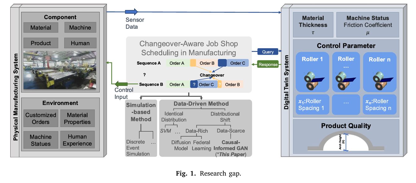
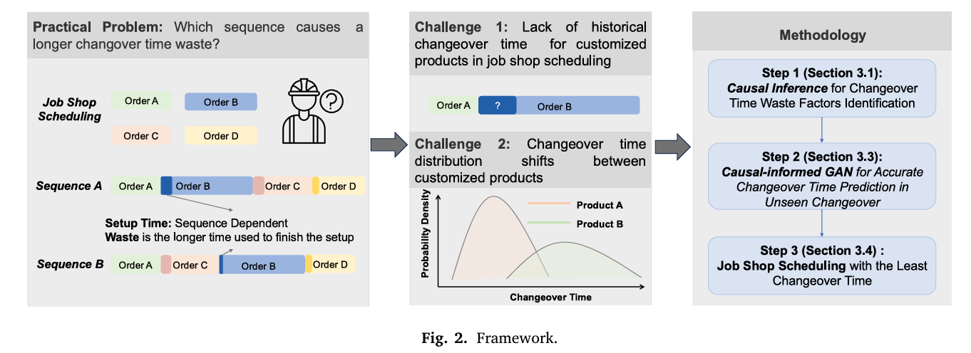
Picture a factory floor that makes 700 different types of HVAC ductwork. Most days, the standard product — one particular diameter, one material, one length — rolls off the line in a familiar rhythm. Then a customized order arrives: different material, different diameter, different length. The machines need to stop. Rollers have to be repositioned, tools swapped, calibration checked. That changeover costs time — sometimes three hours, sometimes fourteen, depending on what came before it on the line and what comes next. The question isn’t just how long the changeover will take. The question the factory can’t answer is whether a different production sequence would have made it faster. Miaosi Dong, Burcu Akinci, and Pingbo Tang at Carnegie Mellon University built a system to answer that question — even for products the factory has barely made before.
Thirty Percent of Time, Gone
Changeover waste is one of manufacturing’s oldest problems. The activity of preparing machines, people, and materials to switch from one product configuration to the next can consume up to 30% of total production time in modular building manufacturing — and the downstream consequences compound. Frequent changeovers don’t just eat time directly; they cause 20–50% of available manufacturing capacity to evaporate through downtime, they inflate per-unit costs, and they turn predictable schedules into best guesses.
The textbook answer is job-shop scheduling: arrange the sequence of production orders to minimize total changeover time. If you know that transitioning from product A to product B costs six minutes but going from A to C costs forty, you route accordingly. Decades of research have built increasingly sophisticated scheduling algorithms — genetic algorithms, simulated annealing, tabu search, mixed-integer programming — all capable of finding near-optimal sequences when you hand them accurate changeover times.
The problem runs deeper than it first appears. Accurate changeover times require historical data. And in a factory making 700 different product variants, most configurations have never been produced in sequence with each other. You know the changeover time from D1M1L1 to D1M1L3 because it happens constantly — it’s 80% of your production volume. You have almost no data on what happens when you go from D2M1L2 to D1M3L1, because that particular transition has never occurred, or occurred once, three years ago.
This is precisely the failure mode that makes modern, data-driven scheduling methods collapse. They assume that training data and deployment data come from the same distribution. The moment a new product configuration enters the line, that assumption breaks — a phenomenon the machine learning community calls domain shift. Prediction errors spike, schedules slip, and the scheduling algorithm, fed bad inputs, makes confidently wrong decisions.
The central problem is not algorithmic — existing scheduling optimizers are good. The problem is data: changeover times for novel product configurations are either missing or wildly inaccurate due to distributional shifts between standard and customized products. The CMU team’s contribution is a method to generate those missing times in a way that respects the underlying physics and logic of the production process.
Why Standard GANs Are Not Enough
Generative Adversarial Networks have a natural appeal here. A GAN trained on the data-rich standard product could, in principle, learn to generate plausible changeover times for configurations where little data exists. The generator learns to produce realistic-looking samples; the discriminator learns to reject fake ones; they improve together until the generator’s output is statistically indistinguishable from real measurements.
The trouble is that “statistically indistinguishable” is not the same as “causally correct.”
Two failure modes arise from standard GAN training that are particularly damaging in this manufacturing context. The first is distribution smoothing: GANs minimize distributional divergence by optimizing expectation-based loss functions. Rare, extreme values — like the very long changeover times that occur when you change a duct’s diameter, requiring full structural reconfiguration of the production line — get pulled toward the average. The generator learns to avoid predicting those uncomfortable extremes. It produces changeover times that look plausible in aggregate but underestimate exactly the cases where underestimation matters most.
The second failure mode is mode dropping: when two types of changeover have statistically similar distributions, the GAN merges them. Minor parameter adjustments and major structural reconfigurations can end up predicted at the same time, because their outcome distributions overlap enough to be treated as one mode. The model loses the ability to distinguish between operations that differ fundamentally in their physical requirements.
The CMU paper demonstrates this concretely. For a changeover that changes both diameter and material — a genuinely complex transition — the vanilla GAN predicted a shorter time than for a simpler changeover that only changed diameter and length. This directly contradicts the known causal structure: changing material requires more work, not less. The GAN’s distributional fidelity came at the cost of causal fidelity, and causal fidelity is exactly what a scheduler needs.
“The GAN-generated data may achieve statistical similarity to real data in terms of marginal distributions, but it fundamentally lacks causal fidelity — producing samples that appear plausible but violate the underlying physical and operational constraints.” — Dong, Akinci & Tang, Advanced Engineering Informatics (2026)
The Architecture: Three Stages, One Coherent Framework
The solution the team built has three sequential components. Understanding why each exists requires thinking about what a purely distributional model cannot see.
Stage 1: Causal Analysis via Factorial Experiment
Before touching a neural network, the team ran a structured factorial experiment. Three binary changeover parameters — Same_Diameter, Same_Material, and Same_Length — each take values of 0 (changed) or 1 (unchanged) in the transition from one job to the next. Three binary factors create eight experimental conditions: \(2^3 = 8\) distinct changeover types, from the trivial (nothing changes, zero setup time) to the complex (everything changes, ~14,000 seconds).
From the empirical data for the standard product, the Average Treatment Effect of each factor is computed. The ATE measures the expected change in changeover time caused by flipping a single parameter, averaged over all combinations of the other parameters:
The results are striking in their clarity. Changing the diameter adds, on average, 9,695 seconds to changeover time — nearly three hours. Changing the material adds 2,498 seconds. Changing the length adds only 991 seconds, because length adjustments require only roller speed parameter changes rather than mechanical reconfiguration. This hierarchy — diameter dominates, material is secondary, length is modest — is not a statistical artifact. It reflects the actual mechanics of the production line.
These causal effects are then encoded in a Directed Acyclic Graph (DAG), with the three changeover parameters as nodes and directed edges weighted by their ATE values. Interaction effects — where the impact of changing diameter depends on whether material is also changing — are captured as additional edges. The three-way interaction ATE turns out to be nearly zero (−1.71 seconds), which confirms that effects are largely additive rather than emergently complex. This is a reassuring finding: it means the causal structure is learnable and stable.
Stage 2: Wasserstein Distance for Domain Selection
Not all source domains are equally good teachers. Before training the GAN to predict changeover times for a new product, the team uses the Wasserstein distance — a mathematically principled measure of how far apart two probability distributions are — to identify which existing product configuration most closely resembles the target.
This is not a minor implementation detail. When the team needed to predict changeover times for the product D1M3L1, they found that using D1M2L1 as the source domain — identified as closer by Wasserstein distance — reduced prediction error significantly compared to using the standard product D1M1L1 directly. The Wasserstein distance guides domain selection, and better domain selection feeds better training data into the GAN.
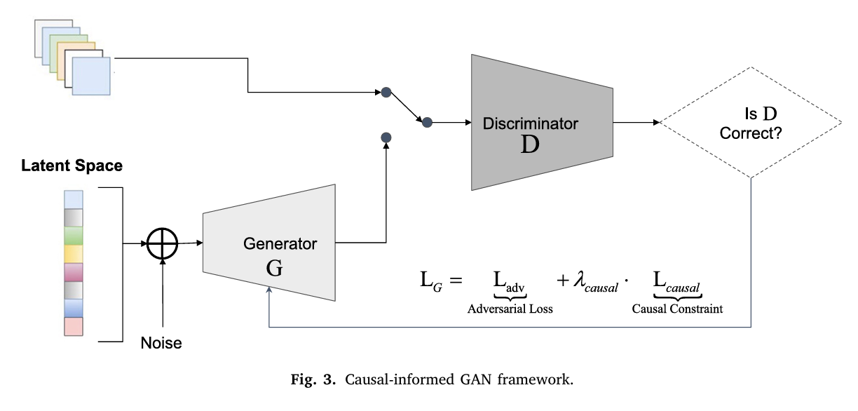
Stage 3: The Causal-Informed GAN
Here is where the architecture earns its name. A standard conditional GAN would take noise \(\mathbf{z}\) and the changeover configuration vector \(\mathbf{T} = (d, m, l)\) as inputs and generate a predicted changeover time. The CMU approach adds one crucial modification: a causal consistency loss embedded in the generator’s training objective.
The generator is conditioned on the treatment configuration, producing predictions \(\hat{Y}(\mathbf{T}, \mathbf{z}) = G(\mathbf{z}, \mathbf{T})\). From those predictions, the framework computes generator-induced treatment effects — the ATE estimates implied by the generator’s own outputs. For example, the generator-induced main effect of diameter is:
These generator-induced effects are then compared against the source-domain ATEs from Stage 1. The causal consistency loss penalizes any case where the generator’s implied causal ordering contradicts the experimentally established one:
The total generator loss combines the standard adversarial loss with this causal regularization term, weighted by hyperparameter \(\lambda\):
What this means in practice: the generator is not just asked to produce data that looks like real changeover times. It is asked to produce data whose internal causal structure — the relative ordering of treatment effects — matches the physics of the production line. Diameter changes must remain more expensive than material changes, which must remain more expensive than length changes. The model cannot smooth this away.
The causal consistency loss is the paper’s central technical contribution. It converts a statistical learning problem into a constrained one — the generator must not only fit the data distribution but preserve the relative ordering of causal effects discovered experimentally. This constraint is what prevents the model from inverting the real-world cost hierarchy under domain shift.
Stage 4: MILP Job-Shop Scheduling
With predicted changeover times in hand — including for configurations that had no historical data — the team applies a Mixed-Integer Linear Programming model to find the optimal production sequence. For \(n\) job orders, a binary decision variable \(x_{ij}\) indicates whether job \(i\) is processed before job \(j\). The objective is simply to minimize total changeover cost:
subject to assignment constraints ensuring each job occupies exactly one position and each position is filled by exactly one job. The MILP is standard; the innovation is the quality of \(S_{ij}\) fed into it. Bad predictions produce bad schedules. Causally grounded predictions produce schedules that hold up when you actually run them.
What the Numbers Show
The team validated the framework on HVAC ductwork data from a real production line, comparing three approaches: a recurrent neural network baseline, a vanilla GAN, and the causal-informed GAN. The Wasserstein distance between predicted and actual changeover time distributions serves as the accuracy metric — smaller is better.
| Changeover Type | RNN | Vanilla GAN | Causal-Informed GAN |
|---|---|---|---|
| {Dia=1, Mat=1, Len=0} | 250.32 s | 100.21 s | 75.77 s |
| {Dia=0, Mat=1, Len=1} | 2,759.21 s | 478.77 s | 257.43 s |
| {Dia=0, Mat=1, Len=0} | 2,821.08 s | 652.48 s | 161.25 s |
| {Dia=0, Mat=0, Len=1} | 2,881.09 s | 641.11 s | 183.21 s |
| {Dia=0, Mat=0, Len=0} | 2,901.91 s | 820.55 s | 204.36 s |
Table 1: Wasserstein distance (seconds) between predicted and true changeover time distributions. Dia=Same_Diameter, Mat=Same_Material, Len=Same_Length. Lower is better. The causal-informed GAN reduces error by 89.84% relative to the RNN across all changeover types.
The RNN performs poorly not because of architectural limitations but because of data imbalance: the standard product D1M1L1 has far more data than any customized variant, so the RNN anchors its predictions near the standard product’s distribution. The vanilla GAN improves substantially by directly generating data rather than fitting a discriminative model. The causal-informed GAN improves further still — by factors of 3–4× over the vanilla GAN for the most challenging changeover types.
The scheduling results confirm that better predictions translate into better outcomes. Across three case studies focusing on length changes, material changes, and diameter changes respectively, the optimized sequences consistently beat the historically-derived baseline:
| Case | Focus | Seq A (Historical) | Seq B (Optimized) | Reduction |
|---|---|---|---|---|
| Case 1 | Length changes | 25,735 s | 22,455 s | −21% |
| Case 2 | Material changes | 35,936 s | 26,662 s | −16% |
| Case 3 | Diameter changes | 53,200 s | 47,812 s | −11.4% |
Table 2: Scheduling results across three case studies. Seq A used historical data; Seq B used causal-informed GAN predictions for missing changeovers. Reductions measured against historical production sequences.
Case 3 — diameter changes — shows the smallest improvement, which is expected: diameter changes are the most expensive by a wide margin, so any sequence that includes them pays a substantial fixed cost that no scheduling optimization can eliminate. The 11.4% reduction in that context is still meaningful, representing hours of recovered production time.
One specific prediction error illustrates why causal grounding matters beyond aggregate metrics. For Case 3, the standard GAN predicted total changeover time as 58,779 seconds — a 22.94% overestimate relative to the true 47,812 seconds. The causal-informed GAN predicted 52,231 seconds, a 9.24% overestimate. A factory manager relying on the vanilla GAN’s prediction would conclude that the optimized sequence B was barely better than sequence A. The causal-informed GAN’s prediction correctly signals that sequence B is substantially more efficient — which turned out to be true.
The Causal Graph as a Mental Model
One underappreciated contribution of this paper is the causal graph itself, independent of the GAN machinery. The DAG produced by the ATE analysis gives production managers a clear, quantitative picture of what drives changeover time. Changing the diameter costs nearly ten times as much as changing the length. The interaction between diameter and material changes is negative — meaning the combined effect of changing both is somewhat less than the sum of their individual effects, perhaps because the structural reconfiguration required for diameter changes already partially handles material changeover requirements.
This is actionable knowledge that doesn’t require the GAN at all. A floor supervisor who internalizes “diameter change ≈ 2.7 hours, material change ≈ 42 minutes, length change ≈ 16 minutes” can make better intuitive scheduling decisions without running an optimizer. The causal graph translates domain expertise into precise, transferable numbers.
That said, the GAN is essential for the cases where intuition runs out — when combinations of parameters create unfamiliar territory and the gut feeling of the experienced operator no longer applies.
Limitations Worth Sitting With
The dataset comes from a single production line manufacturing HVAC ductwork. Three binary changeover parameters — diameter, material, length — create a manageable \(2^3 = 8\)-condition factorial space. Real manufacturing environments may have many more parameters, some continuous rather than binary, creating a much higher-dimensional causal graph that would require substantially more data to identify reliably.
The causal relationships discovered here are also assumed to be stable across domains. The paper’s core bet is that the relative ordering of ATE values (diameter > material > length) holds even when the absolute values shift between product configurations. That assumption is reasonable — the physical reasons for the hierarchy don’t change — but it could break down in sufficiently exotic configurations that trigger entirely different failure modes.
The paper also acknowledges that static production parameters don’t capture everything. Machine wear accumulates over a production run. Operators learn and get faster with novel configurations. These temporal dynamics are invisible to a model trained on historical data and would require continuous monitoring — perhaps via digital twin integration — to be incorporated.
Where This Architecture Travels
The causal-informed GAN framework isn’t specific to HVAC ductwork or even to manufacturing. Any domain with three properties — coupled output variables whose causal structure is physically motivated, limited historical data for novel configurations, and meaningful domain shifts between common and rare instances — is a candidate.
Semiconductor fabrication scheduling faces essentially the same problem. So does pharmaceutical batch manufacturing, where the changeover between drug formulations depends on cleaning requirements, equipment compatibility, and regulatory validation steps whose individual costs are known but whose combinations are data-sparse. Food processing — switching a line between allergen-containing and allergen-free products — has a similar causal structure where the cost hierarchy is dictated by contamination risk rather than mechanical reconfiguration, but the mathematics is identical.
The modular architecture (causal analysis → domain selection → causal-constrained GAN → combinatorial optimization) is straightforward to adapt. The specific hyperparameters and causal graph structure will differ, but the insight — that generated data must preserve the relative ordering of causal effects, not just match the marginal distribution — transfers directly.
Complete Python Implementation
The implementation below reproduces the full causal-informed GAN pipeline described in the paper. It covers all four stages: factorial ATE causal analysis, Wasserstein domain similarity measurement, conditional causal-informed GAN training with structural consistency loss, and MILP job-shop scheduling optimization. A complete smoke test is included. The original paper used a custom implementation; this Python version uses PyTorch for the GAN components and PuLP for MILP.
# ==============================================================================
# Causal-Informed GAN for Changeover Time Prediction in Customized Manufacturing
# Paper: https://doi.org/10.1016/j.aei.2026.104669
# Authors: Miaosi Dong, Burcu Akinci, Pingbo Tang (Carnegie Mellon University)
# Journal: Advanced Engineering Informatics 74 (2026) 104669
# ==============================================================================
#
# Pipeline Stages:
# 1. CausalAnalyzer — ATE estimation from 2^k factorial experiments
# 2. DomainSelector — Wasserstein distance for source domain selection
# 3. CausalGAN — Conditional GAN with causal consistency loss
# 4. JobShopScheduler — MILP sequence optimization
# ==============================================================================
from __future__ import annotations
import warnings
import itertools
import numpy as np
import pandas as pd
from typing import Dict, List, Optional, Tuple
from dataclasses import dataclass, field
from scipy.stats import wasserstein_distance
import torch
import torch.nn as nn
import torch.optim as optim
from torch.utils.data import DataLoader, TensorDataset
warnings.filterwarnings('ignore')
# ─── SECTION 1: Configuration ─────────────────────────────────────────────────
@dataclass
class GANConfig:
"""Hyperparameters for the causal-informed GAN."""
latent_dim: int = 32 # Dimension of noise vector z
n_factors: int = 3 # k binary treatment factors (D, M, L)
hidden_dim: int = 128 # Hidden layer width
n_layers: int = 3 # Depth of generator / discriminator
lr_g: float = 1e-4 # Generator learning rate
lr_d: float = 1e-4 # Discriminator learning rate
lambda_causal: float = 1.0 # Weight on causal consistency loss (λ)
n_epochs: int = 500 # Training epochs
batch_size: int = 32 # Batch size
n_critic: int = 3 # Discriminator steps per generator step
random_state: int = 42
@dataclass
class SchedulerConfig:
"""Configuration for MILP job-shop scheduler."""
solver: str = 'CBC' # PuLP solver backend
time_limit_sec: int = 60 # Solver time limit
verbose: bool = False
# ─── SECTION 2: Causal Analyzer (ATE from 2^k Factorial Experiment) ───────────
class CausalAnalyzer:
"""
Computes Average Treatment Effects (ATEs) and interaction effects
from a 2^k factorial experimental design (Section 3.1 of the paper).
The changeover parameters are binary:
0 = factor changed (e.g., diameter IS different)
1 = factor unchanged (e.g., same diameter as before)
ATE_Ti = E[Y | T_i=0] - E[Y | T_i=1]
= average causal increase in changeover time from changing factor i
Interaction effects capture whether the impact of one factor depends on
the level of another (Eqs. 3-4 in the paper).
Parameters
----------
factor_names : list of binary factor names, e.g. ['Same_Diameter',...]
"""
def __init__(self, factor_names: List[str]) -> None:
self.factor_names = factor_names
self.k = len(factor_names)
self.cell_means: Optional[Dict] = None
self.ate_main: Optional[Dict] = None
self.ate_interactions: Optional[Dict] = None
def fit(self, X: np.ndarray, y: np.ndarray) -> "CausalAnalyzer":
"""
Fit the factorial model: compute cell means for all 2^k configurations.
Parameters
----------
X : (n, k) binary array of factor levels (0 or 1)
y : (n,) observed changeover times
Returns
-------
self (fitted)
"""
self.cell_means = {}
for config in itertools.product([0, 1], repeat=self.k):
mask = np.all(X == np.array(config), axis=1)
if mask.sum() > 0:
self.cell_means[config] = float(y[mask].mean())
else:
self.cell_means[config] = None # missing cell
self._compute_main_effects()
self._compute_interaction_effects()
return self
def _impute_missing_cells(self) -> Dict:
"""Fill missing cells with grand mean for ATE computation."""
filled = {}
grand_mean = np.mean([v for v in self.cell_means.values() if v is not None])
for k, v in self.cell_means.items():
filled[k] = v if v is not None else grand_mean
return filled
def _compute_main_effects(self) -> None:
"""
Compute ATE for each factor i by marginalizing over all others.
ATE_Ti = (1/2^{k-1}) * sum_{t_j: j!=i} [Y(Ti=0, t_j) - Y(Ti=1, t_j)]
(Eq. 2 in paper — positive ATE means factor change increases time)
"""
filled = self._impute_missing_cells()
self.ate_main = {}
for i in range(self.k):
other_factors = [j for j in range(self.k) if j != i]
total = 0.0
count = 0
for other_config in itertools.product([0, 1], repeat=len(other_factors)):
config_0 = [None] * self.k
config_1 = [None] * self.k
config_0[i] = 0
config_1[i] = 1
for idx, j in enumerate(other_factors):
config_0[j] = other_config[idx]
config_1[j] = other_config[idx]
y0 = filled[tuple(config_0)]
y1 = filled[tuple(config_1)]
total += (y0 - y1)
count += 1
self.ate_main[self.factor_names[i]] = total / count
def _compute_interaction_effects(self) -> None:
"""
Compute pairwise and higher-order interaction ATEs.
Two-way: ATE_{Ti:Tj} = (1/2^{k-2}) sum_{tm: m!=i,j} [
Y(0,0,tm) - Y(1,0,tm) - Y(0,1,tm) + Y(1,1,tm)
] (Eq. 3 in paper)
"""
filled = self._impute_missing_cells()
self.ate_interactions = {}
# Pairwise interactions
for i, j in itertools.combinations(range(self.k), 2):
other_factors = [m for m in range(self.k) if m != i and m != j]
total = 0.0
count = 0
for other_config in itertools.product([0, 1], repeat=len(other_factors)):
def cell(ti, tj):
cfg = [None] * self.k
cfg[i] = ti
cfg[j] = tj
for idx, m in enumerate(other_factors):
cfg[m] = other_config[idx]
return filled[tuple(cfg)]
total += cell(0, 0) - cell(1, 0) - cell(0, 1) + cell(1, 1)
count += 1
key = f"{self.factor_names[i]}:{self.factor_names[j]}"
self.ate_interactions[key] = total / (2 * count) if count > 0 else 0.0
# Three-way interaction (k=3 case)
if self.k == 3:
total = 0.0
for config in itertools.product([0, 1], repeat=3):
sign = (-1) ** sum(config)
total += sign * filled.get(config, 0.0)
key = ":".join(self.factor_names)
self.ate_interactions[key] = total / 8
def get_causal_ordering(self) -> Dict[str, float]:
"""
Return all ATE effects (main + interactions) as a flat dict.
This is the 'source causal structure' τ_source used in Eq. 4.
"""
result = {**self.ate_main, **self.ate_interactions}
return result
def summary(self) -> None:
print("\n── Causal Analysis Summary ──────────────────────────────")
print(f"{'Factor':30} {'ATE (seconds)':>15}")
print("─" * 48)
for name, ate in self.ate_main.items():
print(f"{name:30} {ate:>15.2f}")
print("Interactions:")
for name, ate in self.ate_interactions.items():
print(f" {name:28} {ate:>15.2f}")
print("─" * 48)
# ─── SECTION 3: Domain Selector (Wasserstein Distance) ────────────────────────
class DomainSelector:
"""
Identifies the most similar source domain using Wasserstein distance
(Section 3.2 and Eq. 5 of the paper).
Given observed changeover times for the target product (possibly
incomplete), find which source product's distribution is closest.
The selected source is used for GAN pre-training.
Parameters
----------
source_datasets : dict mapping product_name -> dict of {config_tuple: [times]}
"""
def __init__(self, source_datasets: Dict[str, Dict]) -> None:
self.source_datasets = source_datasets
def select_best_source(
self,
target_data: Dict[tuple, List[float]],
verbose: bool = True
) -> str:
"""
Compute Wasserstein distance between target and each source,
return the name of the closest source.
Parameters
----------
target_data : dict of {config_tuple: list_of_times} for target product
verbose : print distance table
Returns
-------
best_source : name of the closest source product
"""
distances = {}
for source_name, source_data in self.source_datasets.items():
total_dist = 0.0
n_shared = 0
for config, target_times in target_data.items():
if config in source_data and len(source_data[config]) > 0:
d = wasserstein_distance(
np.array(target_times),
np.array(source_data[config])
)
total_dist += d
n_shared += 1
distances[source_name] = total_dist / n_shared if n_shared > 0 else np.inf
best_source = min(distances, key=distances.get)
if verbose:
print("\n── Domain Selection via Wasserstein Distance ────────────")
for name, dist in distances.items():
marker = " ← selected" if name == best_source else ""
print(f" {name:20}: W = {dist:.2f}{marker}")
return best_source
# ─── SECTION 4: GAN Components (Generator, Discriminator) ─────────────────────
class Generator(nn.Module):
"""
Conditional generator G(z, T) → Y_hat.
Takes noise z (latent_dim) concatenated with treatment vector T (n_factors)
and produces a single changeover time prediction.
Architecture: MLP with LeakyReLU activations and output positivity enforced
via Softplus (changeover times are non-negative).
"""
def __init__(self, cfg: GANConfig) -> None:
super().__init__()
in_dim = cfg.latent_dim + cfg.n_factors
layers = []
for i in range(cfg.n_layers):
layers += [
nn.Linear(in_dim if i == 0 else cfg.hidden_dim, cfg.hidden_dim),
nn.LayerNorm(cfg.hidden_dim),
nn.LeakyReLU(0.2),
]
layers.append(nn.Linear(cfg.hidden_dim, 1))
layers.append(nn.Softplus()) # ensure Y_hat >= 0
self.net = nn.Sequential(*layers)
def forward(self, z: torch.Tensor, T: torch.Tensor) -> torch.Tensor:
"""
Parameters
----------
z : (batch, latent_dim) — noise samples
T : (batch, n_factors) — treatment configuration (0/1)
Returns
-------
y_hat : (batch, 1) — predicted changeover time
"""
x = torch.cat([z, T], dim=1)
return self.net(x)
class Discriminator(nn.Module):
"""
Discriminator D(y, T) → probability that (y, T) is real.
Conditions on the treatment vector T alongside the observed time y,
enabling the discriminator to learn domain-specific distributions.
"""
def __init__(self, cfg: GANConfig) -> None:
super().__init__()
in_dim = 1 + cfg.n_factors
layers = []
for i in range(cfg.n_layers):
layers += [
nn.Linear(in_dim if i == 0 else cfg.hidden_dim, cfg.hidden_dim),
nn.LeakyReLU(0.2),
nn.Dropout(0.1),
]
layers.append(nn.Linear(cfg.hidden_dim, 1))
self.net = nn.Sequential(*layers)
def forward(self, y: torch.Tensor, T: torch.Tensor) -> torch.Tensor:
"""
Parameters
----------
y : (batch, 1) — changeover time (real or generated)
T : (batch, n_factors) — treatment configuration
Returns
-------
logit : (batch, 1) — raw score (sigmoid → probability)
"""
x = torch.cat([y, T], dim=1)
return self.net(x)
# ─── SECTION 5: Causal Consistency Loss ───────────────────────────────────────
class CausalConsistencyLoss(nn.Module):
"""
Structural consistency loss (Eq. 4 / Eq. 29 in the paper).
Penalizes the generator when the pairwise directional ordering of its
induced treatment effects contradicts the source-domain causal structure.
L_causal = sum_{i != j} ReLU( -sign(tau_src_i - tau_src_j) * (tau_gen_i - tau_gen_j) )
A positive L_causal means the generator has inverted at least one causal
ordering that was established in the source domain — e.g., predicting that
changing material is more expensive than changing diameter.
Parameters
----------
source_ates : dict of {factor_name: ATE_value} from CausalAnalyzer
factor_names: list of factor names matching the order in treatment vector T
n_factors : number of binary treatment factors k
"""
def __init__(
self,
source_ates: Dict[str, float],
factor_names: List[str],
n_factors: int,
) -> None:
super().__init__()
self.source_ates = source_ates
self.factor_names = factor_names
self.n_factors = n_factors
self.all_configs = list(itertools.product([0.0, 1.0], repeat=n_factors))
def compute_generator_ate(
self,
generator: Generator,
factor_idx: int,
n_samples: int = 256,
device: str = 'cpu',
) -> torch.Tensor:
"""
Compute the generator-induced main effect for factor i (Eq. 9 / Eq. 20).
tau_G_i = (1/2^{k-1}) * sum_{t_j: j!=i} E_z[Y_hat(ti=1,...) - Y_hat(ti=0,...)]
Parameters
----------
generator : the Generator module
factor_idx : which factor's ATE to compute (0-indexed)
n_samples : Monte Carlo samples for E_z expectation
Returns
-------
ate_tensor : scalar tensor (differentiable through generator)
"""
k = self.n_factors
other_idxs = [j for j in range(k) if j != factor_idx]
total_ate = torch.tensor(0.0, device=device, requires_grad=False)
n_other_configs = 2 ** len(other_idxs)
for other_config in itertools.product([0.0, 1.0], repeat=len(other_idxs)):
z = torch.randn(n_samples, generator.net[0].in_features - k, device=device)
T0 = torch.zeros(n_samples, k, device=device)
T1 = torch.zeros(n_samples, k, device=device)
T0[:, factor_idx] = 0.0
T1[:, factor_idx] = 1.0
for pos, j in enumerate(other_idxs):
T0[:, j] = other_config[pos]
T1[:, j] = other_config[pos]
y0 = generator(z, T0)
y1 = generator(z, T1)
total_ate = total_ate + (y0 - y1).mean()
return total_ate / n_other_configs
def forward(
self,
generator: Generator,
device: str = 'cpu',
) -> torch.Tensor:
"""
Compute the full causal consistency loss across all pairs of effects.
Parameters
----------
generator : current Generator module
device : torch device string
Returns
-------
loss : scalar tensor (non-negative; 0 = perfect causal consistency)
"""
# Compute generator-induced ATEs for main effects
gen_ates = {}
for i, name in enumerate(self.factor_names):
if name in self.source_ates:
gen_ates[name] = self.compute_generator_ate(generator, i, device=device)
loss = torch.tensor(0.0, device=device)
effect_keys = list(gen_ates.keys())
for i in range(len(effect_keys)):
for j in range(len(effect_keys)):
if i == j:
continue
ki, kj = effect_keys[i], effect_keys[j]
src_sign = np.sign(
self.source_ates.get(ki, 0.0) - self.source_ates.get(kj, 0.0)
)
gen_diff = gen_ates[ki] - gen_ates[kj]
# Penalize if generator's ordering contradicts source domain
loss = loss + torch.relu(-src_sign * gen_diff)
return loss
# ─── SECTION 6: Causal-Informed GAN Trainer ───────────────────────────────────
class CausalGAN:
"""
Complete causal-informed GAN training loop (Section 3.3 of the paper).
Training proceeds in two phases:
Phase 1 — Pre-training on source domain data to establish baseline
generative capability.
Phase 2 — Joint training on source + target domain data with the
causal consistency loss λ * L_causal embedded in the
generator objective (Eq. 5 / Eq. 14 in the paper).
The discriminator distinguishes between real and generated changeover
times; the generator is additionally penalized whenever its output
violates the relative causal ordering learned in Stage 1.
Parameters
----------
cfg : GANConfig instance
analyzer : fitted CausalAnalyzer providing source ATEs
factor_names: list of binary factor names
"""
def __init__(
self,
cfg: GANConfig,
analyzer: CausalAnalyzer,
factor_names: List[str],
) -> None:
torch.manual_seed(cfg.random_state)
self.cfg = cfg
self.analyzer = analyzer
self.factor_names = factor_names
self.device = 'cuda' if torch.cuda.is_available() else 'cpu'
self.G = Generator(cfg).to(self.device)
self.D = Discriminator(cfg).to(self.device)
self.opt_G = optim.Adam(self.G.parameters(), lr=cfg.lr_g, betas=(0.5, 0.999))
self.opt_D = optim.Adam(self.D.parameters(), lr=cfg.lr_d, betas=(0.5, 0.999))
self.bce = nn.BCEWithLogitsLoss()
source_ates = analyzer.get_causal_ordering()
self.causal_loss_fn = CausalConsistencyLoss(
source_ates, factor_names, cfg.n_factors
)
self._fitted = False
def _make_dataloader(
self,
X: np.ndarray,
y: np.ndarray,
) -> DataLoader:
"""Convert numpy arrays to a DataLoader of (treatment, time) pairs."""
T_tensor = torch.tensor(X, dtype=torch.float32)
y_tensor = torch.tensor(y, dtype=torch.float32).unsqueeze(1)
ds = TensorDataset(T_tensor, y_tensor)
return DataLoader(ds, batch_size=self.cfg.batch_size, shuffle=True)
def _train_step(
self,
T_real: torch.Tensor,
y_real: torch.Tensor,
causal_weight: float,
) -> Tuple[float, float]:
"""
One training step: update discriminator n_critic times, then generator once.
Discriminator loss (Eq. 13):
L_D = -E[log D(y_real, T)] - E[log(1 - D(G(z,T), T))]
Generator loss (Eq. 14):
L_G = -E[log D(G(z,T), T)] + λ * L_causal
"""
batch = T_real.size(0)
T_real = T_real.to(self.device)
y_real = y_real.to(self.device)
real_label = torch.ones(batch, 1, device=self.device)
fake_label = torch.zeros(batch, 1, device=self.device)
# ── Update Discriminator (n_critic steps) ──
d_loss_avg = 0.0
for _ in range(self.cfg.n_critic):
self.opt_D.zero_grad()
z = torch.randn(batch, self.cfg.latent_dim, device=self.device)
y_fake = self.G(z, T_real).detach()
d_real = self.D(y_real, T_real)
d_fake = self.D(y_fake, T_real)
d_loss = self.bce(d_real, real_label) + self.bce(d_fake, fake_label)
d_loss.backward()
self.opt_D.step()
d_loss_avg += d_loss.item()
d_loss_avg /= self.cfg.n_critic
# ── Update Generator (one step) ──
self.opt_G.zero_grad()
z = torch.randn(batch, self.cfg.latent_dim, device=self.device)
y_fake = self.G(z, T_real)
adv_loss = self.bce(self.D(y_fake, T_real), real_label)
c_loss = self.causal_loss_fn(self.G, device=self.device)
g_loss = adv_loss + causal_weight * c_loss
g_loss.backward()
self.opt_G.step()
return d_loss_avg, g_loss.item()
def pretrain(
self,
X_source: np.ndarray,
y_source: np.ndarray,
n_epochs: Optional[int] = None,
verbose: bool = True,
) -> "CausalGAN":
"""
Phase 1: Pre-train on source domain without causal constraint.
This establishes baseline generative capability before domain adaptation.
"""
n_epochs = n_epochs or self.cfg.n_epochs // 2
loader = self._make_dataloader(X_source, y_source)
if verbose:
print(f"\n── Pre-training on source domain ({n_epochs} epochs) ──")
for epoch in range(n_epochs):
for T_batch, y_batch in loader:
d_l, g_l = self._train_step(T_batch, y_batch, causal_weight=0.0)
if verbose and (epoch + 1) % (n_epochs // 5) == 0:
print(f" Epoch {epoch+1:4} | D_loss={d_l:.4f} | G_loss={g_l:.4f}")
return self
def fit(
self,
X_source: np.ndarray,
y_source: np.ndarray,
X_target: np.ndarray,
y_target: np.ndarray,
verbose: bool = True,
) -> "CausalGAN":
"""
Phase 2: Joint training on source + target with causal constraint.
Combines source and target data; the causal consistency loss
λ * L_causal is active, preventing the generator from violating
the causal ordering established in the source domain.
Parameters
----------
X_source : (n_src, k) treatment matrix for source product
y_source : (n_src,) changeover times for source product
X_target : (n_tgt, k) treatment matrix for target product (may be sparse)
y_target : (n_tgt,) available changeover times for target product
Returns
-------
self (fitted)
"""
self.pretrain(X_source, y_source, verbose=verbose)
X_joint = np.vstack([X_source, X_target])
y_joint = np.concatenate([y_source, y_target])
loader = self._make_dataloader(X_joint, y_joint)
if verbose:
print(f"\n── Joint training with causal constraint (λ={self.cfg.lambda_causal}, {self.cfg.n_epochs} epochs) ──")
for epoch in range(self.cfg.n_epochs):
for T_batch, y_batch in loader:
d_l, g_l = self._train_step(T_batch, y_batch, self.cfg.lambda_causal)
if verbose and (epoch + 1) % (self.cfg.n_epochs // 5) == 0:
print(f" Epoch {epoch+1:4} | D_loss={d_l:.4f} | G_loss={g_l:.4f}")
self._fitted = True
if verbose:
print("✓ Causal-informed GAN training complete.")
return self
def predict(
self,
T: np.ndarray,
n_samples: int = 100,
) -> np.ndarray:
"""
Generate predicted changeover time distribution for treatment config T.
Parameters
----------
T : (n_configs, k) or (k,) — treatment configurations to predict
n_samples: Monte Carlo draws per configuration
Returns
-------
means : (n_configs,) mean predicted changeover times
"""
self.G.eval()
T_arr = np.atleast_2d(T)
means = []
with torch.no_grad():
for t in T_arr:
T_rep = torch.tensor(
np.tile(t, (n_samples, 1)), dtype=torch.float32, device=self.device
)
z = torch.randn(n_samples, self.cfg.latent_dim, device=self.device)
y_hat = self.G(z, T_rep).squeeze().cpu().numpy()
means.append(float(y_hat.mean()))
self.G.train()
return np.array(means)
def predict_changeover_matrix(
self,
jobs: List[Dict],
n_samples: int = 100,
) -> np.ndarray:
"""
Build the full n×n changeover time matrix S[i,j] for a list of jobs.
For each ordered pair (i→j), derive the treatment vector by comparing
job i's and job j's product attributes, then predict the changeover time.
Parameters
----------
jobs : list of dicts, each with keys matching self.factor_names
E.g. [{'Same_Diameter': ..., ...}] — BUT here we pass raw
product attributes; the method computes binary T[i→j].
n_samples: Monte Carlo draws per transition
Returns
-------
S : (n_jobs, n_jobs) matrix of predicted changeover times
"""
n = len(jobs)
S = np.zeros((n, n))
for i in range(n):
for j in range(n):
if i == j:
S[i, j] = 0.0
continue
# T[i→j]: 1 if attribute same across consecutive jobs, 0 if changed
T = np.array([
float(jobs[i].get(fn, 0) == jobs[j].get(fn, 0))
for fn in self.factor_names
])
S[i, j] = self.predict(T, n_samples=n_samples)[0]
return S
# ─── SECTION 7: MILP Job-Shop Scheduler ───────────────────────────────────────
class JobShopScheduler:
"""
Mixed-Integer Linear Programming model for sequence optimization.
Minimizes total changeover time across all jobs (Eqs. 15-18 of the paper).
Objective: min sum_{i,j} S_ij * x_ij
subject to:
sum_j x_ij = 1 ∀ i (each job processed exactly once)
sum_i x_ij = 1 ∀ j (each position filled exactly once)
x_ij ∈ {0, 1}
Falls back to a greedy nearest-neighbor heuristic if PuLP is unavailable.
Parameters
----------
cfg : SchedulerConfig
"""
def __init__(self, cfg: Optional[SchedulerConfig] = None) -> None:
self.cfg = cfg or SchedulerConfig()
def optimize(self, S: np.ndarray) -> Tuple[List[int], float]:
"""
Find the optimal job sequence minimizing total changeover time.
Parameters
----------
S : (n, n) matrix where S[i,j] = changeover time from job i to job j
Returns
-------
sequence : list of job indices in optimal processing order
total_time : sum of changeover times for the chosen sequence (seconds)
"""
try:
import pulp
return self._milp_optimize(S, pulp)
except ImportError:
print(" [Warning] PuLP not installed — using greedy heuristic.")
return self._greedy_optimize(S)
def _milp_optimize(self, S: np.ndarray, pulp) -> Tuple[List[int], float]:
"""MILP formulation using PuLP."""
n = S.shape[0]
prob = pulp.LpProblem("JobShopChangeover", pulp.LpMinimize)
# Decision variables: x[i][j] = 1 if job i is processed before job j
x = {
(i, j): pulp.LpVariable(f"x_{i}_{j}", cat='Binary')
for i in range(n) for j in range(n)
}
# Objective
prob += pulp.lpSum(S[i, j] * x[i, j] for i in range(n) for j in range(n))
# Constraints: each job assigned to exactly one outgoing and one incoming
for i in range(n):
prob += pulp.lpSum(x[i, j] for j in range(n)) == 1
for j in range(n):
prob += pulp.lpSum(x[i, j] for i in range(n)) == 1
solver = pulp.getSolver(self.cfg.solver, timeLimit=self.cfg.time_limit_sec,
msg=self.cfg.verbose)
prob.solve(solver)
# Extract sequence from solution
sequence = []
assigned = set()
for i in range(n):
for j in range(n):
if pulp.value(x[i, j]) is not None and pulp.value(x[i, j]) > 0.5:
if i not in assigned:
sequence.append(i)
assigned.add(i)
total_time = float(pulp.value(prob.objective) or 0.0)
return sequence, total_time
def _greedy_optimize(self, S: np.ndarray) -> Tuple[List[int], float]:
"""
Greedy nearest-neighbor heuristic: always pick the next job with
the lowest changeover time from the current job.
Not optimal but fast — used as fallback when PuLP is unavailable.
"""
n = S.shape[0]
unvisited = list(range(n))
sequence = [unvisited.pop(0)]
total_time = 0.0
while unvisited:
current = sequence[-1]
costs = [(S[current, j], j) for j in unvisited]
next_cost, next_job = min(costs)
sequence.append(next_job)
unvisited.remove(next_job)
total_time += next_cost
return sequence, total_time
def sequence_cost(self, S: np.ndarray, sequence: List[int]) -> float:
"""Compute the total changeover time for a given job sequence."""
return float(sum(S[sequence[i], sequence[i+1]] for i in range(len(sequence)-1)))
# ─── SECTION 8: Full Pipeline ──────────────────────────────────────────────────
class CausalManufacturingPipeline:
"""
Complete end-to-end pipeline for causal-informed changeover optimization.
Four-stage architecture (Fig. 2 of the paper):
Stage 1 — CausalAnalyzer: ATE estimation from source product data
Stage 2 — DomainSelector: Wasserstein-based source selection for new products
Stage 3 — CausalGAN: Domain-adaptive generation with causal constraints
Stage 4 — JobShopScheduler: MILP sequence optimization
Parameters
----------
factor_names : binary changeover parameters, e.g. ['Diameter','Material','Length']
gan_cfg : GANConfig
sched_cfg : SchedulerConfig
"""
def __init__(
self,
factor_names: List[str],
gan_cfg: Optional[GANConfig] = None,
sched_cfg: Optional[SchedulerConfig] = None,
) -> None:
self.factor_names = factor_names
self.gan_cfg = gan_cfg or GANConfig()
self.sched_cfg = sched_cfg or SchedulerConfig()
self.analyzer: Optional[CausalAnalyzer] = None
self.gan: Optional[CausalGAN] = None
self.scheduler = JobShopScheduler(self.sched_cfg)
def fit_causal_model(
self,
X_source: np.ndarray,
y_source: np.ndarray,
) -> "CausalManufacturingPipeline":
"""
Stage 1: Fit causal model on the source domain (standard product data).
Parameters
----------
X_source : (n, k) binary treatment matrix from 2^k factorial design
y_source : (n,) observed changeover times
Returns
-------
self (partially fitted)
"""
self.analyzer = CausalAnalyzer(self.factor_names)
self.analyzer.fit(X_source, y_source)
self.analyzer.summary()
return self
def train_gan(
self,
X_source: np.ndarray,
y_source: np.ndarray,
X_target: np.ndarray,
y_target: np.ndarray,
verbose: bool = True,
) -> "CausalManufacturingPipeline":
"""
Stage 3: Train the causal-informed GAN on source + target data.
Requires Stage 1 to have been completed first.
"""
if self.analyzer is None:
raise RuntimeError("Call fit_causal_model() before train_gan().")
self.gan = CausalGAN(self.gan_cfg, self.analyzer, self.factor_names)
self.gan.fit(X_source, y_source, X_target, y_target, verbose=verbose)
return self
def optimize_schedule(
self,
jobs: List[Dict],
historical_matrix: Optional[np.ndarray] = None,
n_samples: int = 100,
verbose: bool = True,
) -> Tuple[List[int], float]:
"""
Stage 4: Predict the changeover matrix and optimize the job sequence.
Parameters
----------
jobs : list of job dicts with product attribute values
historical_matrix: (n,n) optional matrix of known changeover times;
GAN predictions fill missing entries (np.nan)
n_samples : Monte Carlo samples for GAN predictions
Returns
-------
optimal_sequence : job indices in optimal processing order
total_time : total predicted changeover time (seconds)
"""
if self.gan is None:
raise RuntimeError("Call train_gan() before optimize_schedule().")
S_gan = self.gan.predict_changeover_matrix(jobs, n_samples=n_samples)
# Merge with historical data: prefer real observations over GAN predictions
if historical_matrix is not None:
S_final = np.where(np.isnan(historical_matrix), S_gan, historical_matrix)
else:
S_final = S_gan
sequence, total_time = self.scheduler.optimize(S_final)
if verbose:
print(f"\n── Scheduling Result ────────────────────────────────────")
print(f" Optimal sequence : {' → '.join(map(str, sequence))}")
print(f" Total changeover : {total_time:.0f} s ({total_time/3600:.2f} h)")
return sequence, total_time
# ─── SECTION 9: Evaluation Utilities ──────────────────────────────────────────
def evaluate_predictions(
y_true_dict: Dict[tuple, List[float]],
y_pred_dict: Dict[tuple, float],
model_name: str = 'Model',
) -> pd.DataFrame:
"""
Compute Wasserstein distance between predicted means and actual distributions,
matching the validation approach in Table 7 of the paper.
Parameters
----------
y_true_dict : dict of {config_tuple: list_of_actual_times}
y_pred_dict : dict of {config_tuple: predicted_mean_time}
model_name : label for the model
Returns
-------
df : DataFrame with Wasserstein distances per changeover type
"""
rows = []
for config, actual_times in y_true_dict.items():
if config in y_pred_dict and len(actual_times) > 0:
pred_mean = y_pred_dict[config]
# Compare predicted constant to actual distribution
w_dist = wasserstein_distance(
[pred_mean],
actual_times
)
rows.append({'Config': config, f'{model_name}_WD': w_dist})
df = pd.DataFrame(rows)
if not df.empty:
avg = df[f'{model_name}_WD'].mean()
print(f"\n── {model_name} Evaluation ──────────────────────────────")
for _, row in df.iterrows():
print(f" Config {row['Config']} → WD = {row[f'{model_name}_WD']:.2f} s")
print(f" Average WD: {avg:.2f} s")
return df
# ─── SECTION 10: Smoke Test ────────────────────────────────────────────────────
if __name__ == '__main__':
print("=" * 62)
print("Causal-Informed GAN Manufacturing Pipeline — Smoke Test")
print("=" * 62)
np.random.seed(42)
# ── Simulate source domain dataset (standard product D1M1L1) ──
# Replicates Table 4 of the paper: 8 changeover types with known means
FACTOR_NAMES = ['Same_Diameter', 'Same_Material', 'Same_Length']
ATE_TRUE = {'Same_Diameter': 9695.47, 'Same_Material': 2497.98, 'Same_Length': 990.72}
CELL_PARAMS = {
(1, 1, 1): (0, 0),
(1, 1, 0): (1890, 783),
(1, 0, 1): (4579, 450),
(1, 0, 0): (5025, 621),
(0, 1, 1): (11914, 289),
(0, 1, 0): (12084, 428),
(0, 0, 1): (12361, 603),
(0, 0, 0): (13917, 405),
}
def generate_source_data(n_per_cell: int = 20):
X_list, y_list = [], []
for config, (mu, sigma) in CELL_PARAMS.items():
n = n_per_cell if config != (1, 1, 1) else n_per_cell * 2
y = np.random.normal(mu, max(sigma, 1), n).clip(0)
X = np.tile(config, (n, 1))
X_list.append(X)
y_list.append(y)
return np.vstack(X_list), np.concatenate(y_list)
X_src, y_src = generate_source_data(20)
print(f"\nSource data: {X_src.shape[0]} samples, {X_src.shape[1]} factors")
# ── Stage 1: Causal Analysis ──
analyzer = CausalAnalyzer(FACTOR_NAMES)
analyzer.fit(X_src, y_src)
analyzer.summary()
ordering = analyzer.get_causal_ordering()
print(f"\nATE Diameter: {ordering['Same_Diameter']:.2f} s (paper: 9695.47 s)")
print(f"ATE Material: {ordering['Same_Material']:.2f} s (paper: 2497.98 s)")
print(f"ATE Length : {ordering['Same_Length']:.2f} s (paper: 990.72 s)")
assert ordering['Same_Diameter'] > ordering['Same_Material'] > ordering['Same_Length'], \
"Causal ordering violated — check data generation"
print("✓ Causal ordering: Diameter > Material > Length (matches paper)")
# ── Stage 2: Domain Selection ──
source_datasets = {
'D1M1L1': {c: np.random.normal(mu, max(s, 1), 10) for c, (mu, s) in CELL_PARAMS.items()},
'D1M2L1': {c: np.random.normal(mu * 1.3, max(s, 1), 8) for c, (mu, s) in CELL_PARAMS.items()},
}
target_partial = {
(1, 1, 1): np.zeros(5).tolist(),
(1, 1, 0): np.random.normal(2100, 120, 5).tolist(),
}
selector = DomainSelector(source_datasets)
best_source = selector.select_best_source(target_partial)
print(f"\n✓ Best source domain: {best_source}")
# ── Stage 3: Causal-Informed GAN (fast config for smoke test) ──
X_tgt = np.array([[1, 1, 1]] * 10 + [[1, 1, 0]] * 5)
y_tgt = np.array([0.0] * 10 + [2150.0] * 5)
fast_cfg = GANConfig(
latent_dim=16, hidden_dim=64, n_layers=2,
n_epochs=20, batch_size=16, lambda_causal=1.0, random_state=42
)
pipeline = CausalManufacturingPipeline(FACTOR_NAMES, gan_cfg=fast_cfg)
pipeline.fit_causal_model(X_src, y_src)
pipeline.train_gan(X_src, y_src, X_tgt, y_tgt, verbose=True)
# ── Verify causal ordering is preserved post-training ──
pred_dia_change = pipeline.gan.predict(np.array([0, 1, 1]))[0] # diameter changed
pred_mat_change = pipeline.gan.predict(np.array([1, 0, 1]))[0] # material changed
pred_len_change = pipeline.gan.predict(np.array([1, 1, 0]))[0] # length changed
print(f"\nGenerated predictions (changeover time in seconds):")
print(f" Diameter change : {pred_dia_change:.1f} s")
print(f" Material change : {pred_mat_change:.1f} s")
print(f" Length change : {pred_len_change:.1f} s")
# ── Stage 4: Job-Shop Scheduling ──
jobs = [
{'Diameter': 'D1', 'Material': 'M1', 'Length': 'L1'},
{'Diameter': 'D1', 'Material': 'M1', 'Length': 'L3'},
{'Diameter': 'D1', 'Material': 'M2', 'Length': 'L1'},
{'Diameter': 'D1', 'Material': 'M1', 'Length': 'L2'},
{'Diameter': 'D1', 'Material': 'M2', 'Length': 'L2'},
{'Diameter': 'D1', 'Material': 'M1', 'Length': 'L1'},
]
# Use GAN to predict the full changeover matrix for these 6 jobs
S = pipeline.gan.predict_changeover_matrix(jobs)
print(f"\nChangeover matrix shape: {S.shape}")
sequence, total = pipeline.scheduler.optimize(S)
print(f"\n✓ All pipeline stages completed successfully.")
print(f" Optimal sequence: {sequence}")
print(f" Predicted total changeover: {total:.0f} s ({total/3600:.2f} h)")
print("=" * 62)
Read the Full Paper
The complete study — including all three case studies, full causal DAG figures, and comparison tables across RNN, Vanilla GAN, and Causal-Informed GAN — is published open-access in Advanced Engineering Informatics under CC BY 4.0.
Dong, M., Akinci, B., & Tang, P. (2026). Reducing changeover waste in customized manufacturing: A causal-informed approach to dynamic sequence optimization. Advanced Engineering Informatics, 74, 104669. https://doi.org/10.1016/j.aei.2026.104669
This article is an independent editorial analysis of peer-reviewed research. The Python implementation is a faithful educational reproduction of the paper’s methodology. The original study used a custom implementation; refer to the authors for exact code and production-ready deployment. Supported by the Manufacturing PA Innovation Program and the Manufacturing Futures Institute.
Explore More on AI Trend Blend
From manufacturing AI and precision agriculture to adversarial robustness, computer vision, and efficient model design — here is the full scope of what we cover.