
- GNSS spoofing detection
- CORS networks
- Graph signal processing
- Ionospheric TEC
- Integrity monitoring
- Intelligent transportation
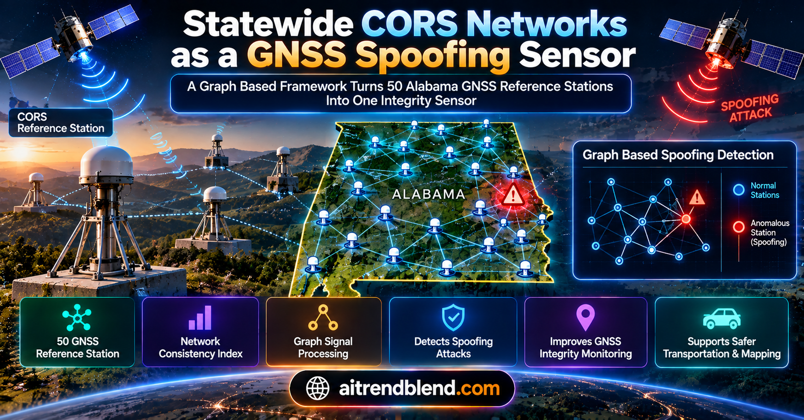
A grading crew on an Alabama highway project trusts a stream of centimeter level corrections to steer its machines. Those corrections come from a statewide network of permanent GNSS reference stations that the Department of Transportation owns and maintains. If one of those stations started reporting a subtly wrong picture of the sky, because of a faulty receiver, local radio interference or a deliberate spoofer, who would notice?
A team from the University of Alabama and Clemson University argues the answer is already sitting in the data. In a new preprint on arXiv, Minhaj Uddin Ahmad and colleagues treat the 50 station Alabama DOT network as a single sensor spread across the state, where every station is checked against its neighbors rather than against its own past. They call it the Network Consistency Framework, and on two ordinary summer days it picked out two stations that did not fit.
Key points
- The framework represents a statewide network of continuously operating reference stations as a graph, with each station a node and its six nearest stations as neighbors.
- Four metrics score each station against its neighborhood, and a robust composite called the Network Consistency Index combines them across observables.
- It uses ionospheric quantities, day over day change in vertical total electron content and the rate of TEC index, because these vary smoothly across tens of kilometers and are hard for a spoofer to fake.
- On 5 and 6 July 2026 data from 50 Alabama stations, two stations stood out, ALMJ with an index of 10.6 and AL84 with 4.1, against a network median of 0.76.
- No new hardware is needed, but the demonstration covers only two quiet days and no controlled spoofing test, so detection rates remain unmeasured.
The problem with checking receivers one at a time
GNSS signals are astonishingly weak by the time they reach the ground. The paper puts the received power on the order of \(10^{-16}\) watts, and civil signals carry no authentication except for Galileo’s newer Navigation Message Authentication. That combination is what makes spoofing cheap. Researchers showed back in 2008 that a portable transmitter could broadcast a counterfeit constellation and steer a receiver toward positions or times of the attacker’s choosing. The EU STRIKE3 project later logged hundreds of thousands of interference incidents, and more than 10 percent of them were deliberate.
For transportation the stakes are concrete. A spoofed signal feeding an automated vehicle, a survey of record or a timing system is a failure of safety and trust at the same time. And the infrastructure involved is not small. A 2025 Caltrans survey cited in the paper found that ten of thirteen responding agencies own or co own their reference stations, with system costs of roughly one to ten million dollars and annual budgets near one million.
Most integrity methods look inward. Receiver Autonomous Integrity Monitoring checks whether a receiver’s own measurements are self consistent. Interference monitors on national reference networks, such as Sweden’s SWEPOS and Finland’s FinnRef, compare each station’s signal to noise ratio against a model of that station’s history. Both work within their scope. The trouble is what they cannot see. A receiver that has already been fully captured by a self consistent spoofer has little internal reason to complain, and a fault that looks normal compared with a station’s own past will never be flagged.
The authors point to a property these networks have simply by existing. Their stations share one geographic environment, so they should agree on quantities that vary smoothly over the region. That agreement is a free cross check nobody has been using for integrity.
The gap between short and continental baselines
Here is where it gets interesting. Multi receiver spoofing detection is not new. Tippenhauer and colleagues showed in 2011 that an attacker can drive many receivers to one common location, but cannot easily preserve their true relative formation. Later detectors compared positions or double differenced pseudoranges across receivers a few tens of meters to about a kilometer apart, and in 2025 Chen and Wang improved that approach with a spatial distribution statistic.
Those methods share a design choice. Double differencing cancels satellite clock errors and ionospheric and tropospheric delays, because on short baselines those delays are common to every receiver. The paper’s core observation is that the quantity those methods throw away is exactly the signal it wants to keep. At the 21 to 55 kilometer spacing of a statewide network, atmospheric delay does not cancel between neighbors. It varies smoothly, and that smooth field becomes the reference against which each station is judged.
At the other end, the large networks behind Satellite Based Augmentation Systems and Precise Point Positioning already screen out stations with bad residuals. But they are continental and sparse, and they discard the anomalous station to protect the correction product rather than localizing what happened. The Alabama network sits in the middle regime, dense enough to localize and wide enough that atmospheric structure survives.
Short baseline spoofing detectors ask whether receivers agree with a single counterfeit transmitter. This framework asks whether a station agrees with the geophysical field its neighbors describe. The two ideas are complementary, not competing.
Why a spoofer would struggle to hide
The paper lays out what an adversary would need to do to stay invisible. At every affected station, simultaneously, it would have to reproduce the exact geometric range and range rate to each satellite for that station’s surveyed coordinates and clock. It would have to inject the correct position specific atmospheric delays, so that the reconstructed ionosphere matches the smooth surface the neighbors define. And it would have to keep code and carrier phase mutually consistent on every frequency as the real satellites move.
Physical range makes this harder still. Citing Chen and Wang’s link budget analysis, the authors note that an omnidirectional transmitter at 0 dBm reliably overwhelms a receiver only within about 120 meters, and capture becomes possible at most a few kilometers out. Both figures sit far below the median station spacing, so one terrestrial spoofer cannot plausibly capture two stations at once. Evading the network would take coordinated, mutually consistent spoofing with a separate transmitter near each station.
Think about what this actually requires. The attack stops being a gadget problem and becomes a regional operation, which is a very different threat model.
Which measurements can be compared across stations
Not every quantity a station reports makes sense to interpolate from its neighbors, and the paper is careful about this. It splits observables into two classes.
Class A observables are governed by the atmosphere over the region rather than by hardware at any one site. They form smooth fields, so a station’s value should be close to what its neighbors imply. Class B observables, such as carrier to noise density, code multipath and single point positioning scatter, are dominated by the local antenna, receiver and radio environment. Neighbors carry no information about them, so they are excluded from the spatial test. They are still kept, because a drop in carrier to noise density is the main way jamming shows up, and because they offer independent evidence when a spatial flag needs explaining.
Total electron content
The first Class A observable comes from the ionosphere. Free electrons delay code signals by an amount that depends on frequency, so differencing two code pseudoranges removes geometry, clocks and the troposphere and leaves the ionospheric term plus hardware biases.
Here \(b_r\) and \(b^s\) are the receiver and satellite differential code biases, hardware delays that differ between frequencies and stay stable for hours to days. A thin shell model at 350 kilometers converts slant TEC to vertical TEC, with a 25 degree elevation mask.
Absolute VTEC needs the biases to be known, which is a nuisance. The authors avoid it neatly by taking the day over day change, ΔVTEC. Subtracting two days cancels the satellite bias and also the receiver bias as long as that bias stays stable. A receiver whose bias jumps between days breaks that assumption, and as we will see, that is exactly how one of the flagged stations gave itself away.
Rate of TEC index
The second Class A observable is ROTI, the standard deviation of the rate of change of slant TEC over the analysis window. It rises during geomagnetic storms, but under quiet conditions it is small and close to uniform across a region.
Four ways to measure disagreement
The network becomes an undirected graph. Stations are nodes, edges connect each station to its \(k = 6\) nearest neighbors in map projection, and edge weights fall with distance. The authors chose six as the smallest neighborhood that keeps the graph connected for this geometry while staying local enough that one bad neighbor cannot dominate a median. The setup follows standard graph signal processing, with each observable treated as a signal living on the graph.
Neighborhood residual
The simplest measure is the gap between a station and the median of its neighbors. The median, rather than the mean, keeps a single anomalous neighbor from dragging the reference.
Spatial gradient
To catch abrupt spatial change, the method fits a local plane to the neighborhood by distance weighted least squares and takes the slope magnitude, in field units per kilometer.
A subtle point is that a local disturbance inflates the gradient throughout the surrounding neighborhood, not only at the disturbed station. So this metric does not identify the culprit. It identifies the ring of stations the culprit affects.
Prediction residual
The primary anomaly score predicts each station from the others and measures the miss. It uses the same inverse distance weighted interpolator that drives the map products, with power two and the eight nearest contributors, in leave one out fashion.
This is not a small distinction. Because \(\hat f_i\) never uses \(f_i\), a faulty station cannot mask its own fault. That property is why the composite index is built on \(P_i\) and not on the other three. The authors add that kriging could replace inverse distance weighting without changing the framework.
Graph smoothness
The fourth metric looks at the whole network. Using Gaussian edge weights with a scale set to the median nearest neighbor distance, the graph Laplacian gives a Dirichlet energy that grows as nearby stations disagree, plus a per station share of that energy.
One number per station
To put metrics and observables on the same scale, each is converted to a robust z score using the network median and the median absolute deviation, so that an absolute value of three or more marks an outlier under a Gaussian assumption. The Network Consistency Index is then the weighted quadratic mean of the prediction residual z scores across the chosen Class A observables.
With default weights of one, a station consistent with its neighborhood scores near one, and a station whose observables jointly depart from what the network predicts scores well above it. The authors are explicit that the index measures spatial consistency and nothing more. A high score means a station disagrees with its surroundings. It does not say whether the reason is interference, a spoofer, a receiver fault or an antenna problem.
Rather than testing whether a station appears anomalous relative to its own history, we test whether it appears anomalous relative to its spatial neighborhood at the same epoch.Ahmad et al., arXiv:2608.08831
Two days of Alabama data
The demonstration uses archived observations from the 50 station Alabama DOT network for 5 and 6 July 2026. Each day holds 2,880 epochs per station at a 30 second interval, in RINEX 3.04 format, with carrier phase, code, Doppler and carrier to noise measurements for GPS, GLONASS, Galileo and BeiDou. The network streams 1 Hz data in real time over NTRIP, but the agency allows one user only one stream, so the study worked from the archive. The authors note the method would translate to real time if all 50 streams were available at once.
The first result is almost mundane, and the paper is right to report it. Forty nine stations delivered every expected epoch, and AL92 delivered 99.9 percent, a single gap of about two and a half minutes. Station AL62 was fine on both study days but went down on 7 July. An operational system has to screen outages like that first, or a dead station would be misread as a spatial anomaly.
A coherent field with one hole in it
Across the state, ΔVTEC between the two days changed by a smooth 1.2 TECU at the median, spanning roughly negative two to positive three TECU, with small gradients and a total graph Dirichlet energy of 139. That is what a healthy Class A field looks like.
Station AL84 in west central Alabama broke the pattern. Its ΔVTEC of negative 2.1 TECU sat against a neighborhood near positive one TECU. That produced the largest neighborhood residual in the network, with an absolute z of 5.8, the largest prediction residual at negative 3.6 TECU with an absolute z of 5.5, and the highest local graph energy. The gradient map lit up the ring of neighbors around it, stations ALGR and ALAS, which carried the next largest residuals. The four metrics told a consistent story, the residuals pointing at the station and the gradient outlining the neighborhood it disturbed.
Evidence from outside the spatial test backs this up. AL84 showed jumps in carrier to noise density, a Class B observable, and on the following day it carried an offset of about 14 TECU that was uniform across all satellites. That uniformity is the fingerprint of a change in receiver differential code bias, the exact assumption ΔVTEC depends on. So AL84 looks like a genuine receiver side anomaly. The authors are careful to add that a similar signature could come from intentional interference or spoofing, and that confirming the cause would require spectrum monitoring or signal level analysis.
The composite index
ROTI was quiet across the state, with a median of 0.09 TECU per minute, apart from one station. Combining both observables, the statewide index had a median of 0.76 and a 90th percentile of 2.2. Two stations stood well clear of that background.
| Station | NCI | Dominant contributor | External evidence |
|---|---|---|---|
| ALMJ | 10.6 | ROTI, |z| = 15 | ROTI 0.29 TECU per minute, 3.2 times the network median |
| AL84 | 4.1 | ΔVTEC, Pi = −3.6 TECU | Carrier to noise jump, 14 TECU all satellite bias jump on 7 July |
| ALGR | 3.1 | ΔVTEC, |z| = 4.4 | Not independent, neighbor of AL84 |
| ALCH | 2.7 | ROTI, |z| = 3.8 | None available |
| AL90 | 2.4 | ROTI, |z| = 3.4 | None available |
| ALAS | 2.2 | ΔVTEC, |z| = 3.1 | Not independent, neighbor of AL84 |
| ALTU | 2.2 | ROTI, |z| = 2.8 | None available |
| AL92 | 2.0 | ROTI, |z| = 2.7 | None available |
Reproduced from Table 1 of the preprint, the eight least spatially consistent stations over 5 and 6 July 2026.
ALMJ is the more puzzling case. Its ROTI of 0.29 TECU per minute stands against quiet neighbors in every direction out to tens of kilometers, so it is local rather than a regional ionospheric event. But nothing outside the framework explains it, and ALMJ sits in a sparse corner of the network, with its nearest neighbor roughly 42 kilometers away against a median spacing near 21 kilometers. The authors therefore label it a lower confidence detection. It is a real, isolated anomaly whose cause could be a receiver or antenna fault, local interference or a spoofing attempt.
The framework did what it promised. It localized two stations using only data the network already collects. What it cannot yet do is say why they disagree, and it is less certain near the sparse edges of the network.
How this connects to graph learning
Readers who follow our graph neural networks coverage will recognize the toolkit. A graph Laplacian, a Dirichlet energy and leave one out prediction on a k nearest neighbor graph are the same building blocks that sit underneath message passing networks. The difference is that nothing here is learned. Every weight comes from geometry and a fixed interpolation rule.
That is a sensible choice for a first demonstration. There are no labeled spoofing events to train on, and a hand built index is easier to explain to a transportation agency than a black box score. But it also points to obvious next steps. Our piece on graph curvature and community detection shows how edge level geometry can reveal where one region ends and another begins, which could help the framework adapt its neighborhoods near sparse boundaries. And the robust prototype ideas in HPGRL’s noise resistant graph classification hint at how a learned model might tolerate a few bad nodes without losing the overall picture.
On the security side, the framework fits the pattern we described in our review of adversarial machine learning for intrusion detection. The strongest defenses exploit a constraint the attacker cannot easily satisfy. Here that constraint is geography.
What this means for transportation agencies
The practical pitch is strong. Agencies already pay for these networks, and the framework runs on observations they already archive. It needs no new antennas, no new receivers and no external correction product. For departments of transportation facing growing reliance on precise positioning for machine guidance, mapping and connected vehicles, a continuously running regional cross check is cheap insurance.
There are organizational hurdles. Real time operation would need all station streams at once, which the Alabama network’s single stream policy currently prevents. And a flag is only useful if someone owns the follow up, whether that is checking a receiver’s bias history, dispatching a spectrum survey or coordinating with neighboring states. The authors suggest cross state data sharing to strengthen coverage near borders, which is where their own detection confidence drops.
Honest limitations
The study covers two days of nominal, geomagnetically quiet operation. Seasonal effects, storm conditions and long term variability are untested, and during a geomagnetic storm, ROTI and TEC gradients rise sharply and unevenly, which could either mask anomalies or produce false ones.
There was no controlled spoofing or jamming experiment. The two detections are naturally occurring anomalies, one plausibly explained by a receiver bias change and one unexplained. So the paper demonstrates localization, not detection rates. We do not yet know how often the index would catch a real spoofer, or how often it would raise false alarms over months of operation.
Network geometry matters. ALMJ’s case shows that confidence falls where stations are sparse, and the median and inverse distance weighting choices assume enough neighbors to outvote one bad value.
The ΔVTEC observable assumes stable receiver biases between days. A bias jump will be flagged, which is useful for maintenance, but it means some flags will reflect hardware housekeeping rather than threats.
Finally, this is an arXiv preprint submitted in August 2026 and not yet peer reviewed. The method is clearly described and the numbers are modest in their claims, but independent replication on other state networks would strengthen it considerably.
PyTorch implementation of the Network Consistency Framework
Below is a complete reimplementation written from the equations in the paper. It includes the ionospheric observables, the k nearest neighbor graph, all four consistency metrics, the robust z scores and the composite index, wrapped as a PyTorch module. The smoke test builds a synthetic 50 station network, injects a ΔVTEC drop and a ROTI spike similar to the AL84 and ALMJ cases, and checks that both are ranked at the top. One note on signs. The paper writes the code difference in Eq. 2 as \(\rho_1 – \rho_2\). The code uses \(\rho_2 – \rho_1\), consistent with Eq. 1, so that the larger delay on the lower frequency gives positive TEC.
# ncf.py
# Network Consistency Framework (NCF) and Network Consistency Index (NCI)
# Reimplementation in PyTorch of the method described in
# Ahmad, Dasgupta, Irfan, Rahman, Chowdhury and Bandi, arXiv:2608.08831 (2026).
# Stations are graph nodes, a Class A observable (dVTEC or ROTI) is a graph signal.

from __future__ import annotations
import math
import torch

TECU = 1e16                     # electrons per m^2
K_ION = 40.308                  # first order ionospheric constant
C_LIGHT = 299_792_458.0
R_EARTH_KM = 6371.0


# ------------------------------------------------------------------
# 1. Ionospheric observables (Eqs. 1 to 3)
# ------------------------------------------------------------------
def stec_from_code(p1: torch.Tensor, p2: torch.Tensor, f1: float, f2: float,
                   dcb_rx: float = 0.0, dcb_sat: float = 0.0) -> torch.Tensor:
    """Slant TEC in TECU from the geometry free code combination (Eqs. 1, 2).
    p1, p2 are pseudoranges in meters, DCBs in seconds. Written as p2 - p1 so
    that the larger L2 delay gives positive TEC. Use float64 for pseudoranges."""
    factor = (f1 ** 2 * f2 ** 2) / (K_ION * (f1 ** 2 - f2 ** 2))
    return factor * ((p2 - p1) - C_LIGHT * (dcb_rx + dcb_sat)) / TECU


def vtec_from_stec(stec: torch.Tensor, elev_deg: torch.Tensor,
                   shell_h_km: float = 350.0, mask_deg: float = 25.0) -> torch.Tensor:
    """Thin shell mapping (Eq. 3). Returns NaN below the elevation mask."""
    el = torch.deg2rad(elev_deg)
    sin_z = R_EARTH_KM / (R_EARTH_KM + shell_h_km) * torch.cos(el)
    cos_z = torch.sqrt(1.0 - sin_z ** 2)
    v = stec * cos_z
    return torch.where(elev_deg >= mask_deg, v, torch.full_like(v, float("nan")))


def roti(stec_series: torch.Tensor, dt_min: float = 0.5) -> torch.Tensor:
    """Rate of TEC index, std of dSTEC/dt over the window (TECU per minute).
    stec_series has shape [..., T]."""
    rot = torch.diff(stec_series, dim=-1) / dt_min
    return torch.nanmean((rot - torch.nanmean(rot, -1, keepdim=True)) ** 2, -1).sqrt()


# ------------------------------------------------------------------
# 2. Graph construction
# ------------------------------------------------------------------
def pairwise_km(pos: torch.Tensor) -> torch.Tensor:
    """pos [N, 2] projected coordinates in km."""
    return torch.cdist(pos, pos)


def knn(dist: torch.Tensor, k: int) -> torch.Tensor:
    """Indices [N, k] of the k nearest neighbors, excluding self."""
    d = dist.clone()
    d.fill_diagonal_(float("inf"))
    return torch.topk(d, k, largest=False).indices


# ------------------------------------------------------------------
# 3. The four spatial consistency metrics (Eqs. 4 to 11)
# ------------------------------------------------------------------
def neighborhood_residual(f: torch.Tensor, nbr: torch.Tensor) -> torch.Tensor:
    """R_i = f_i - median_{j in N(i)} f_j   (Eq. 4)."""
    return f - f[nbr].median(dim=1).values


def spatial_gradient(f: torch.Tensor, pos: torch.Tensor, nbr: torch.Tensor,
                     dist: torch.Tensor) -> torch.Tensor:
    """G_i = sqrt(b^2 + c^2) from a distance weighted local plane fit (Eqs. 5, 6)."""
    n, k = nbr.shape
    dxy = pos[nbr] - pos[:, None, :]                            # [N, k, 2]
    A = torch.cat([torch.ones(n, k, 1, dtype=f.dtype), dxy], -1) # [N, k, 3]
    w = 1.0 / dist.gather(1, nbr).clamp_min(1e-6)               # [N, k]
    W = torch.diag_embed(w)
    y = f[nbr].unsqueeze(-1)                                    # [N, k, 1]
    AtW = A.transpose(1, 2) @ W
    coef = torch.linalg.solve(AtW @ A, AtW @ y).squeeze(-1)     # [N, 3] = a, b, c
    return torch.linalg.vector_norm(coef[:, 1:], dim=-1)


def prediction_residual(f: torch.Tensor, dist: torch.Tensor,
                        n_contrib: int = 8, p: float = 2.0) -> torch.Tensor:
    """Leave one out IDW prediction residual P_i = f_i - f_hat_i (Eqs. 7, 8).
    f_i never enters its own prediction, so a faulty station cannot mask itself."""
    idx = knn(dist, n_contrib)
    w = dist.gather(1, idx).clamp_min(1e-6) ** (-p)
    f_hat = (w * f[idx]).sum(1) / w.sum(1)
    return f - f_hat


def graph_energy(f: torch.Tensor, dist: torch.Tensor):
    """Gaussian weighted graph Dirichlet energy (Eqs. 9 to 11).
    Returns total J = f^T L f and per station contributions E_i."""
    d_off = dist.clone()
    d_off.fill_diagonal_(float("inf"))
    sigma = d_off.min(1).values.median()                         # median NN distance
    W = torch.exp(-dist ** 2 / (2 * sigma ** 2))
    W.fill_diagonal_(0.0)
    L = torch.diag(W.sum(1)) - W
    J = f @ L @ f
    E = (W * (f[:, None] - f[None, :]) ** 2).sum(1)
    return J, E


# ------------------------------------------------------------------
# 4. Robust normalization and the composite index (Eqs. 12, 13)
# ------------------------------------------------------------------
def robust_z(x: torch.Tensor) -> torch.Tensor:
    med = x.median()
    mad = (x - med).abs().median().clamp_min(1e-12)
    return (x - med) / (1.4826 * mad)


class NetworkConsistencyFramework(torch.nn.Module):
    """Scores every station of a reference network against its neighbors.

    forward(observables) takes a dict {name: tensor[N]} of Class A fields
    and returns per station metrics plus the NCI."""

    def __init__(self, pos_km: torch.Tensor, k: int = 6, n_idw: int = 8,
                 idw_power: float = 2.0, weights: dict | None = None):
        super().__init__()
        self.register_buffer("pos", pos_km.double())
        self.register_buffer("dist", pairwise_km(self.pos))
        self.register_buffer("nbr", knn(self.dist, k))
        self.n_idw, self.p = n_idw, idw_power
        self.weights = weights or {}

    def metrics(self, f: torch.Tensor) -> dict:
        f = f.double()
        J, E = graph_energy(f, self.dist)
        return {
            "R": neighborhood_residual(f, self.nbr),
            "G": spatial_gradient(f, self.pos, self.nbr, self.dist),
            "P": prediction_residual(f, self.dist, self.n_idw, self.p),
            "E": E,
            "J": J,
        }

    def forward(self, observables: dict) -> dict:
        out, num, den = {}, 0.0, 0.0
        for name, f in observables.items():
            m = self.metrics(f)
            z_p = robust_z(m["P"]).abs()                          # z_{i,m} = |z(P_i^(m))|
            v = float(self.weights.get(name, 1.0))
            num = num + v * z_p ** 2
            den += v
            out[name] = {**m, "zR": robust_z(m["R"]), "zP": z_p}
        out["NCI"] = torch.sqrt(num / den)                        # Eq. 13
        return out


def flag(nci: torch.Tensor, names: list[str], threshold: float = 3.0):
    """Stations whose NCI exceeds the |z| >= 3 outlier convention, worst first."""
    order = torch.argsort(nci, descending=True)
    return [(names[i], round(float(nci[i]), 2)) for i in order if nci[i] >= threshold]


# ------------------------------------------------------------------
# 5. Smoke test on a synthetic 50 station network
# ------------------------------------------------------------------
if __name__ == "__main__":
    torch.manual_seed(0)
    N = 50
    # Stations scattered over a 300 km by 500 km state sized box
    pos = torch.stack([torch.rand(N) * 300, torch.rand(N) * 500], 1)
    names = [f"ST{i:02d}" for i in range(N)]

    # Smooth dVTEC field around +1.2 TECU with a gentle regional trend
    dvtec = 1.2 + 0.004 * (pos[:, 0] - 150) - 0.002 * (pos[:, 1] - 250)
    dvtec = dvtec + 0.05 * torch.randn(N)
    # Quiet ROTI near 0.09 TECU/min
    roti_field = 0.09 + 0.004 * torch.randn(N)

    # Inject two local anomalies like the paper's AL84 and ALMJ cases
    bad_dvtec, bad_roti = 7, 23
    dvtec[bad_dvtec] = -2.1                  # isolated dVTEC drop
    roti_field[bad_roti] = 0.29              # isolated ROTI spike

    ncf = NetworkConsistencyFramework(pos, k=6)
    res = ncf({"dVTEC": dvtec, "ROTI": roti_field})
    nci = res["NCI"]

    flagged = flag(nci, names)
    print("Median NCI :", round(float(nci.median()), 2))
    print("Flagged    :", flagged[:5])
    print("dVTEC J    :", round(float(res["dVTEC"]["J"]), 2))

    top2 = {n for n, _ in flagged[:2]}
    assert {names[bad_dvtec], names[bad_roti]} == top2, top2
    assert float(nci.median()) < 1.5
    assert res["dVTEC"]["P"][bad_dvtec] < -2.0     # large negative prediction residual

    # Observable helpers
    f1, f2 = 1575.42e6, 1227.60e6
    p1 = torch.tensor([20_000_000.0], dtype=torch.float64)
    p2 = p1 + 3.0                                    # 3 m of extra L2 delay
    stec = stec_from_code(p1, p2, f1, f2)
    assert 25 < float(stec) < 35                     # about 28.6 TECU
    v = vtec_from_stec(stec, torch.tensor([60.0]))
    assert float(v) < float(stec)
    assert torch.isnan(vtec_from_stec(stec, torch.tensor([10.0]))).all()
    r = roti(torch.cumsum(torch.randn(3, 120) * 0.05, -1))
    assert r.shape == (3,) and (r > 0).all()
    print("All smoke tests passed.")
Conclusion
This paper makes a simple idea precise. A statewide reference network is not fifty separate receivers that happen to share an owner. It is one sensor spread across a state, and its stations define what each other should be seeing. By turning that intuition into a graph with four consistency metrics and a robust composite index, the authors isolated two anomalous Alabama stations from nothing more than routine archived data.
The conceptual shift is in where the reference comes from. Receiver level monitors compare a station with itself, and national interference monitors compare it with its own history. This framework compares a station with its neighbors at the same moment, using the very atmospheric structure that short baseline spoofing detectors deliberately cancel. That makes the baseline instantaneous and hard to fake, since an attacker would need to reproduce a smooth regional ionosphere at several widely separated sites at once.
The approach should transfer well beyond Alabama and beyond GNSS. Any network of sensors observing a spatially smooth field, air quality monitors, weather stations, seismic arrays or traffic loop detectors, can use the same recipe of leave one out prediction, robust z scores and graph energy to find the node that does not belong. The classification of observables into interpolable and site specific classes is a useful discipline for any of those settings.
The limits are clear and the authors state them. Two quiet days, no controlled attack, lower confidence near sparse edges and no attribution of cause. The next steps they propose, longer observation periods, controlled spoofing experiments using a virtual reference station and real time operation on a live network, are exactly the ones needed to turn a promising demonstration into an operational tool.
For agencies that have already spent millions building these networks, the message is encouraging. The integrity monitor may already be installed. It just has to be asked the right question.
Frequently asked questions
What is a CORS network?
A continuously operating reference station network is a set of permanent GNSS receivers with antennas at precisely surveyed points. State transportation agencies use them to deliver centimeter level real time corrections for surveying, construction machine guidance, mapping and other precise positioning work.
How does the Network Consistency Framework detect GNSS spoofing?
It treats the stations as a graph and checks whether each station’s ionospheric measurements agree with what its neighbors predict at the same moment. A spoofer or local fault affects one site, so that station stops matching the smooth field its neighbors describe and receives a high consistency score.
What is the Network Consistency Index?
It is a single score per station, the weighted quadratic mean of robust z scores of the leave one out prediction residual across the chosen observables. Stations consistent with their neighbors score near one, and stations that disagree score well above it.
Why use ionospheric TEC instead of signal strength?
Total electron content varies smoothly over tens of kilometers, so neighbors can predict it. Signal strength depends mostly on local hardware and surroundings, so neighbors cannot predict it, although it remains useful as independent evidence when a station is flagged.
Did the framework detect an actual spoofing attack?
No. It flagged two naturally occurring anomalies in Alabama data. One, AL84, is consistent with a receiver bias change, and the other, ALMJ, remains unexplained. The authors did not run a controlled spoofing experiment.
Does the method need new hardware?
No. It runs on observations that statewide networks already collect and archive. Real time operation does require access to all station data streams at the same time.
Read the original research
The preprint includes the full maps, equations and station table.
arXiv abstract page Full paper PDFAhmad, M. U., Dasgupta, S., Irfan, M. S., Rahman, M., Chowdhury, M., and Bandi, T. N. Treating Statewide CORS Networks as Spatially Distributed Sensors for GNSS Integrity Monitoring under Unintentional and Deliberate Threats. arXiv:2608.08831, submitted 10 August 2026. The University of Alabama and Clemson University. Supported by the National Center for Transportation Cybersecurity and Resiliency (TraCR) and the National Science Foundation.
This analysis is based on the published paper and an independent evaluation of its claims. The PyTorch code is an independent reimplementation from the paper’s equations, not the authors’ software.