
Key points
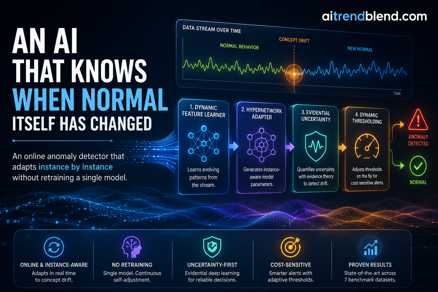
- Researchers built DyMETER, an online anomaly detection framework that adjusts itself to shifting data patterns, known as concept drift, without retraining or fine tuning a model.
- Its core trick is a hypernetwork, a small network that generates targeted parameter adjustments for the main detector at the moment each new data point arrives, rather than updating the whole model through gradient descent.
- A dedicated evolution controller, built on evidential deep learning, estimates how uncertain the model is about each incoming instance, so the expensive adaptation step only fires when genuinely needed.
- A fixed anomaly threshold is replaced with one that continuously recalibrates itself using recent score history plus a dedicated pool of borderline, uncertain cases.
- Across 23 real world and synthetic benchmarks, spanning financial style logs, network intrusion data, supercomputer logs, insect sensor readings, and image streams, DyMETER beat 18 established baselines in the large majority of test conditions while running faster than most of them.
- The authors are candid that the method assumes historical training data reasonably represents what normal looks like at the start, an assumption that can strain in especially noisy or data scarce settings.
When the definition of normal keeps moving
Anomaly detection sounds simple in the abstract, learn what normal looks like, then flag anything that deviates from it. Streaming data breaks that simplicity almost immediately. In a live data stream, normal itself keeps changing. Market trends shift, seasons come and go, new trading strategies emerge, and a transaction pattern that would have looked suspicious last month might be entirely ordinary today. This phenomenon, concept drift, is the central obstacle in what researchers call online anomaly detection, identifying anomalous instances in real time as the stream’s own statistical character evolves underneath the model.
The paper draws a distinction worth sitting with. A concept change point is not automatically an anomaly. A shift from ordinary weekday transactions to holiday transactions redefines what counts as normal, it does not itself signal fraud. The actual anomalies are the deviations that occur within that new, redefined normal, a fraudulent transaction concealed among a flood of legitimate holiday purchases, for instance. A good online detector therefore has to do two things at once, track how normal is drifting, and keep spotting genuine outliers inside whatever normal currently looks like, all without a human resetting its thresholds by hand.
Why the existing playbook falls short
Incremental methods retrain too often
One established approach builds an initial detector and updates it repeatedly as new data streams in. This works, but it is expensive. Constant retraining or fine tuning consumes compute and, worse, tends to lag behind fast moving drift precisely when responsiveness matters most.
Ensemble methods buy flexibility at a steep price
A second family keeps a pool of models, each specialized for a different concept, and combines their outputs. This sidesteps some of the retraining cost, but effectiveness is capped by how large and diverse that pool can practically get, and maintaining many models simultaneously eats memory and compute in its own right.
Drift aware architectures are narrow specialists
A newer line of work bakes adaptation directly into the model’s architecture. These systems can be effective, but they are typically tailored to a specific style of drift and lack flexibility once conditions depart from what they were designed to handle. Across all three traditions, the authors identify the same underlying gaps, adaptation is usually driven by coarse window level signals rather than judged instance by instance, models require continuous tuning or multiple copies rather than efficient adjustment at inference time, and decision boundaries are typically fixed, blind to subtle, context dependent anomalies that only make sense relative to the current concept.
Four parts working as one coordinated system
DyMETER answers each of those three gaps with a dedicated, tightly coupled module.
The static detector, a memory of what normal usually looks like
The Static Concept aware Detector is an autoencoder trained on a slice of historical data to capture the stream’s dominant, recurring patterns. It compresses each input into a latent vector and reconstructs it, and the model learns by minimizing the squared difference between input and reconstruction. Because it becomes a reliable identity mapper for the concepts it was trained on, elevated reconstruction error on new data becomes a first, simple signal of possible anomaly.
The evolution controller, deciding when adaptation is actually warranted
Reconstruction error alone gets unreliable once the data drifts away from what the static detector learned, which is exactly when a naive system would either overreact or miss the shift entirely. The Intelligent Evolution Controller addresses this using evidential deep learning, a framework that models a Dirichlet distribution over class probabilities rather than a single point estimate, giving the system an explicit measure of how confident, or how ignorant, it is about a given input.
Alpha is the Dirichlet evidence vector the controller produces for an input, and Phi is the digamma function. When an input matches previously learned concepts, the evidence stays concentrated and this uncertainty score stays low. When an input comes from a genuinely new concept, the evidence spreads out and the score rises, giving the system an interpretable early warning that something about the data has changed.
The controller is trained using pseudo labels drawn straight from the static detector, poorly reconstructed inputs are labeled as one class, well reconstructed inputs as another, and a focal weighted objective gives extra attention to minority and misclassified cases, since anomalies are by nature rare and imbalanced. Only when this uncertainty score crosses a threshold does the system decide that adaptation is worth the cost, otherwise it leaves the static detector alone.
The dynamic detector, a hypernetwork that nudges the model per instance
When adaptation is warranted, DyMETER does not retrain anything. Instead it uses a hypernetwork, a small network whose job is to generate parameters for a separate, primary network, an idea with roots well outside anomaly detection. Where a conventional hypernetwork generates parameters from a randomly initialized vector with no connection to the actual input, DyMETER’s Dynamic Shift aware Detector conditions that generation directly on the current instance.
A shared encoder processes the current input x, and a small linear layer per network layer extracts a feature vector tied specifically to that instance. Two further linear layers turn that feature vector into a parameter adjustment K for the corresponding layer of the static detector. The static detector’s original weights plus this adjustment become the dynamic detector, re centered toward the new concept for that instance without a single gradient step of retraining.
Because the correction is generated fresh for every incoming instance rather than tuned once for an entire batch or window, the detector can re center itself with a precision that coarser, window level adaptation methods cannot match, all while skipping the computational overhead of actual gradient based fine tuning.
The threshold that moves with the data
A detector is only as good as the line it draws between normal and anomalous, and a fixed line does not survive concept drift intact. DyMETER first turns reconstruction error and concept uncertainty into a single calibrated anomaly score, then maintains two sliding windows to keep the decision boundary current, one tracking the recent distribution of scores for data classified as normal, and a second tracking borderline, uncertain cases sitting close to the current threshold.
Re is the raw reconstruction error and re is a reference error tracked by an exponential moving average, so the score A is reconstruction error rescaled by how uncertain the model is about that instance. The final threshold combines a quantile based baseline, mu superscript zero sub a, with a correction term built from the median score, A sub m, of the borderline window. If that median sits well below the baseline, the threshold rises to guard against missed anomalies, and if it does not, the correction stays small.
Put through 23 benchmarks against 18 rivals
The team tested DyMETER against eighteen established baselines across four families, classic proximity based detectors such as Local Outlier Factor and Isolation Forest, incremental methods including RRCF and MemStream, ensemble methods such as Kitsune and ARCUS, and newer drift aware architectures including D3R, SARAD, and the team’s own earlier system, METER. Evaluation spanned 23 benchmarks, nineteen real world datasets and four synthetic ones, covering financial style transaction logs, network intrusion data from KDDCUP99 and NSL-KDD, supercomputer log data from a BlueGene/L system, insect monitoring sensor data used specifically to simulate controlled drift, several time series benchmarks from the UCR archive and the Numenta anomaly benchmark, and synthetic streams built from MNIST and FMNIST images with engineered abrupt and gradual drift patterns.
| Test setting | What was measured | Headline result |
|---|---|---|
| Discrete setting, unknown drift types, 14 result comparisons | AUCROC and AUCPR against all 18 baselines | Best result in 9 cases, second best in 4 more, top two in 13 of 14 total comparisons |
| Continuous setting, known drift types such as abrupt and incremental | AUCROC across 8 datasets | Best performance on 6 of 8 datasets, an average improvement of 4.1 percentage points over the next best method, the team’s own earlier system METER |
| Synthetic streams built from MNIST and FMNIST | AUCROC under engineered abrupt and gradual drift | Consistently ahead of newer drift aware architectures and its own predecessor, though the ensemble method ARCUS occasionally matched or slightly exceeded it under gradual drift specifically, without matching its overall consistency |
| Inference speed across the same benchmarks | Runtime relative to baseline methods | Inference time under half that of the baseline methods on average, while still delivering superior detection accuracy |
Taking it apart, what each module is actually worth
An ablation study strips DyMETER down piece by piece to see which components are doing the real work. Removing the dynamic, hypernetwork driven detector entirely costs up to 18.1 percent in AUCROC, by far the largest single drop in the study, confirming that instance level parameter adaptation, not just the static detector or the uncertainty signal alone, is the component carrying the most weight. Removing the dynamic thresholding module costs 7.1 percent, showing that recalibrating the decision boundary matters almost as much as recalibrating the detector itself. Swapping the evolution controller’s focal weighted training objective for an ordinary cross entropy loss costs 2.7 percent, a smaller but still meaningful gap attributable to how imbalanced true anomalies are within any real stream.
Two further tests are worth calling out specifically. Swapping the static detector’s plain autoencoder backbone for an LSTM, a 1D convolutional network, or a 1D convolutional network with residual connections each improved results further, by 4.4, 3.1, and 3.8 percentage points respectively, which tells you DyMETER’s benefit comes from its adaptation mechanism rather than being tied to one specific encoder choice. And replacing the hypernetwork’s instance conditioned input with a generic random embedding, the traditional hypernetwork design, produced a clear and significant drop, direct confirmation that conditioning the parameter shift on the actual incoming data point, not just having a hypernetwork at all, is what makes the mechanism work.
Does adapting during deployment actually beat expensive retraining
A separate experiment speaks directly to whether all this online machinery is worth it compared with simply retraining periodically. The team split one dataset into five sequential chunks and ran two experiments, one where the model is retrained offline on each new chunk in turn, and one where it is trained exactly once and left to adapt purely through its online, inference time mechanisms from then on. The purely online version reached an average AUCROC of 0.795 across the later chunks, close to the 0.811 achieved on the very first chunk it saw and comparable overall to the costly, repeatedly retrained version. On two of the later test chunks, the retrained version actually performed worse than the version that was never retrained at all, a reminder that periodic retraining is not a free win and can itself introduce instability into a reconstruction based model.
Watching the model think during an actual drift event
One of the more illustrative results in the paper walks through a single drift event step by step. At one point in a monitored stream, the model shows low uncertainty and correctly calls an incoming sample normal. Shortly after, its concept uncertainty score spikes sharply, an internal signal that the data has started to depart from what the static detector learned, and this triggers the dynamic, hypernetwork driven mode. Immediately after adapting, the model classifies a genuinely normal but unfamiliar looking sample correctly despite the drift. By the time several thousand further samples have passed, the uncertainty score has settled back down, evidence that the model has internalized the new concept rather than merely reacting to it moment by moment. This kind of trace is what the authors mean by interpretability here, not a post hoc explanation bolted onto a black box, but a built in signal that a person monitoring the system can watch rise and fall in step with real events in the stream.
Stress tests, missing data, and a live production pipeline
Beyond the standard benchmarks, the team pushed DyMETER through several deliberately harder conditions. Injecting Gaussian noise into the historical training data, and separately shrinking how much of the true concept that training data actually covers, both degrade performance somewhat, but the decline is modest and smooth rather than a cliff, and DyMETER continues to outperform its strongest baseline throughout. In a more elaborate test, the team concatenated four different insect sensor datasets end to end, creating one long stream that mixes abrupt, gradual, incremental, and recurring drift types back to back. Despite that complexity, DyMETER’s AUCROC stays above 0.785 throughout, with only slight, temporary dips exactly at the points where one drift regime hands off to the next.
Perhaps the most convincing test of practical readiness is that the team did not stop at offline benchmarks at all. They integrated DyMETER as an operator inside Apache Flink, a widely used framework for processing unbounded, real time data streams, and ran it live against one of the insect monitoring datasets. The system sustained a consistently high AUCROC throughout that live run, evidence that the method’s efficiency claims hold up outside a controlled experimental script and inside an actual streaming data pipeline.
Where the authors say the method still falls short
The paper is direct about one structural assumption underneath everything else. DyMETER’s static detector assumes the historical data it starts from is a reasonably faithful sample of what normal looks like. In an especially noisy environment, or one where clean historical data is simply scarce, that starting assumption can be shakier than the method needs it to be. The robustness experiments show the system remains competitive even under those harder conditions, but the authors treat this as an open problem rather than a solved one, and they point to two directions for future work, incorporating self supervised or regularization strategies to make that initial learning phase less dependent on clean historical data, and moving toward proactive adaptation, where the model’s own uncertainty dynamics are used to anticipate a coming drift event before it fully arrives, a step the authors frame as part of a longer term goal of lifelong anomaly detection that keeps working indefinitely as a stream evolves.
Building a simplified DyMETER pipeline in PyTorch
The implementation below sketches the four coupled modules, a static autoencoder detector, an evidential evolution controller estimating concept uncertainty from a Dirichlet distribution, a hypernetwork that generates instance conditioned parameter shifts, and a dynamic thresholding routine built on a sliding window. A smoke test at the end runs the full pipeline on randomly generated dummy data so the code can be verified without any real dataset.
import torch
import torch.nn as nn
import torch.nn.functional as F
import collections

# ----------------------------------------------------------------------
# Static Concept aware Detector, a plain autoencoder
# ----------------------------------------------------------------------
class StaticDetector(nn.Module):
    def __init__(self, input_dim, latent_dim=16):
        super().__init__()
        self.encoder = nn.Sequential(
            nn.Linear(input_dim, 32), nn.ReLU(), nn.Linear(32, latent_dim)
        )
        self.decoder = nn.Sequential(
            nn.Linear(latent_dim, 32), nn.ReLU(), nn.Linear(32, input_dim)
        )

    def forward(self, x):
        z = self.encoder(x)
        y = self.decoder(z)
        return y, z

    def reconstruction_error(self, x):
        y, _ = self.forward(x)
        return ((x - y) ** 2).mean(dim=-1)


# ----------------------------------------------------------------------
# Intelligent Evolution Controller, an evidential classifier
# ----------------------------------------------------------------------
class EvolutionController(nn.Module):
    def __init__(self, input_dim, num_classes=2):
        super().__init__()
        self.net = nn.Sequential(
            nn.Linear(input_dim, 32), nn.ReLU(), nn.Linear(32, num_classes)
        )
        self.num_classes = num_classes

    def forward(self, x):
        evidence = F.softplus(self.net(x))
        alpha = evidence + 1.0
        return alpha

    def concept_uncertainty(self, x):
        alpha = self.forward(x)
        C = self.num_classes
        alpha_sum = alpha.sum(dim=-1, keepdim=True)
        p_hat = alpha / alpha_sum
        entropy = -(p_hat * torch.log(p_hat + 1e-8)).sum(dim=-1)
        digamma_alpha = torch.digamma(alpha + 1.0)
        digamma_sum = torch.digamma(alpha_sum + 1.0)
        expected_term = (p_hat * digamma_alpha).sum(dim=-1)
        uncertainty = expected_term - digamma_sum.squeeze(-1) - entropy
        return uncertainty.abs()

    def focal_loss(self, x, labels, gamma=2.0):
        alpha = self.forward(x)
        alpha_sum = alpha.sum(dim=-1, keepdim=True)
        p_hat = alpha / alpha_sum
        p_true = p_hat.gather(1, labels.unsqueeze(1)).squeeze(1)
        alpha_true = alpha.gather(1, labels.unsqueeze(1)).squeeze(1)
        loss = ((1 - p_true) ** gamma) * (torch.log(alpha_sum.squeeze(-1)) - torch.log(alpha_true))
        return loss.mean()


# ----------------------------------------------------------------------
# Dynamic Shift aware Detector, a hypernetwork that shifts the static detector
# ----------------------------------------------------------------------
class HyperShift(nn.Module):
    def __init__(self, input_dim, target_param_size, hidden=32):
        super().__init__()
        self.shared_encoder = nn.Sequential(nn.Linear(input_dim, hidden), nn.ReLU())
        self.to_shift = nn.Sequential(nn.Linear(hidden, hidden), nn.ReLU(), nn.Linear(hidden, target_param_size))

    def forward(self, x):
        feat = self.shared_encoder(x)
        shift = self.to_shift(feat)
        return shift


def apply_parameter_shift(base_layer, shift_flat):
    # reshape a flat shift vector into the same shape as the layer's weight
    with torch.no_grad():
        shift = shift_flat.view_as(base_layer.weight)
        adjusted_weight = base_layer.weight + shift
    return adjusted_weight


# ----------------------------------------------------------------------
# Dynamic Threshold Optimization, a sliding window based recalibration
# ----------------------------------------------------------------------
class DynamicThreshold:
    def __init__(self, window_size=64, tau=0.95, kappa=0.8):
        self.window_normal = collections.deque(maxlen=window_size)
        self.window_uncertain = collections.deque(maxlen=window_size)
        self.tau = tau
        self.kappa = kappa

    def update(self, score, is_normal, is_uncertain):
        if is_normal:
            self.window_normal.append(score)
        if is_uncertain:
            self.window_uncertain.append(score)

    def current_threshold(self):
        if len(self.window_normal) < 5:
            return float("inf")
        sorted_scores = sorted(self.window_normal)
        idx = int(self.tau * (len(sorted_scores) - 1))
        base_threshold = sorted_scores[idx]
        if len(self.window_uncertain) >= 3:
            median_uncertain = sorted(self.window_uncertain)[len(self.window_uncertain) // 2]
            reg_term = self.kappa * (base_threshold - median_uncertain)
        else:
            reg_term = 0.0
        return base_threshold + reg_term


# ----------------------------------------------------------------------
# Uncertainty calibrated anomaly score
# ----------------------------------------------------------------------
def anomaly_score(recon_error, uncertainty, ref_error, lam=0.6):
    return recon_error * torch.exp(lam * uncertainty * (ref_error - recon_error))


# ----------------------------------------------------------------------
# Smoke test on dummy streaming data, no real dataset required
# ----------------------------------------------------------------------
if __name__ == "__main__":
    torch.manual_seed(0)
    input_dim = 10

    static_detector = StaticDetector(input_dim)
    controller = EvolutionController(input_dim)
    threshold_tracker = DynamicThreshold()

    # train the static detector briefly on dummy "historical" normal data
    optimizer = torch.optim.Adam(static_detector.parameters(), lr=1e-2)
    history = torch.randn(200, input_dim)
    for epoch in range(50):
        optimizer.zero_grad()
        y, _ = static_detector(history)
        loss = F.mse_loss(y, history)
        loss.backward()
        optimizer.step()

    ref_error = static_detector.reconstruction_error(history).max().item()
    hyper = HyperShift(input_dim, target_param_size=static_detector.encoder[0].weight.numel())

    # stream a mix of normal and drifted dummy instances
    stream = torch.cat([torch.randn(20, input_dim), torch.randn(20, input_dim) * 3 + 2], dim=0)

    results = []
    for i in range(stream.shape[0]):
        x = stream[i].unsqueeze(0)
        recon_error = static_detector.reconstruction_error(x)
        uncertainty = controller.concept_uncertainty(x)
        score = anomaly_score(recon_error, uncertainty, torch.tensor(ref_error))
        threshold = threshold_tracker.current_threshold()
        is_anomaly = (score.item() > threshold)
        is_uncertain = uncertainty.item() > 0.3
        threshold_tracker.update(score.item(), is_normal=not is_anomaly, is_uncertain=is_uncertain)
        results.append((i, round(score.item(), 4), round(uncertainty.item(), 4), is_anomaly))

    print("Smoke test complete, first ten stream results")
    for row in results[:10]:
        print(row)
Running this end to end confirms every piece connects, the static detector trains and reconstructs, the evolution controller produces a usable uncertainty signal from the Dirichlet formulation, the anomaly score blends reconstruction error with that uncertainty, and the sliding window threshold updates itself as scores stream in. As with any smoke test on synthetic data, the actual anomaly calls it makes are not meaningful, real deployment needs genuine historical data and the full hypernetwork parameter injection the paper describes, but the structure mirrors DyMETER’s real design closely enough to build from.
Why this design pattern reaches beyond anomaly detection
Strip away the anomaly detection framing and DyMETER is really a demonstration of a more general pattern, decoupling the question of whether a model should adapt from the question of how it should adapt, and answering the first question with a cheap, interpretable uncertainty signal rather than folding both decisions into one expensive retraining loop. Any system that has to operate continuously against a data distribution it does not fully control, a recommendation engine, a fraud pipeline, a monitoring dashboard for industrial sensors, faces some version of this same problem, and the evidence here suggests that instance level, inference time correction can do real work that periodic retraining cannot cheaply match.
The honest limitations matter for anyone evaluating this for production use. The entire framework leans on an assumption that its initial historical data window is a fair representative sample of normal, and while the robustness tests show the system tolerates a fair amount of noise and missing coverage in that initial sample, the authors do not claim the assumption is bulletproof. Teams considering this kind of architecture should weigh how confident they are in their own historical data before assuming the same resilience carries over automatically.
Frequently asked questions
What is online anomaly detection and why is concept drift a problem for it?
Online anomaly detection means spotting unusual data points in a live, continuously arriving stream rather than a fixed dataset. Concept drift is the complication that the definition of normal in that stream keeps changing over time, so a detector tuned to yesterday’s normal can misfire badly on today’s data.
What makes DyMETER different from methods that just retrain periodically?
Instead of retraining or fine tuning the whole model, DyMETER uses a hypernetwork to generate a small, targeted parameter adjustment for each incoming data point at inference time, which the paper shows performs comparably to costly periodic retraining without the recurring cost.
How does the system decide when to adapt versus when to leave the detector alone?
A separate evolution controller, built on evidential deep learning, estimates a concept uncertainty score for each instance. Only when that score crosses a threshold does the system trigger the adaptation mechanism, otherwise the static detector handles the input as usual.
Is a shift in normal behavior itself treated as an anomaly?
No. The paper is explicit that a concept change point is not automatically anomalous. DyMETER separates tracking a shift in normal from identifying genuine outliers within that new normal, so it does not flag every drift event as suspicious.
Does the extra intelligence in DyMETER slow it down?
The paper reports the opposite. Across benchmark datasets, DyMETER’s inference time came in under half that of the baseline methods on average, while still achieving higher detection accuracy, and the added evolution controller and hypernetwork modules added only a few milliseconds of training time and a few megabytes of memory per epoch.
Has this been tested outside of academic benchmarks?
Yes. The authors integrated DyMETER into Apache Flink, a production grade stream processing framework, and ran it live against real sensor data, where it sustained high detection accuracy in an operational, real time pipeline setting.
Read the full paper for every benchmark table, ablation result, and sensitivity study, or explore the released code to reproduce the results yourself.
Zhu, J., Cai, S., Chen, J., Deng, F., Ooi, B. C., and Zhang, W. (2026). Catching every ripple, enhanced anomaly awareness via dynamic concept adaptation. IEEE Transactions on Pattern Analysis and Machine Intelligence, volume 48, issue 8. Available at doi.org/10.1109/TPAMI.2026.3682661. Code released at github.com/zjiaqi725/DyMETER. This work extends the authors’ earlier VLDB paper on the METER framework.
This analysis is based on the published paper and an independent evaluation of its claims.