
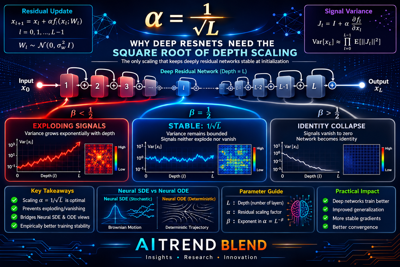
- ResNets add a scaling factor in front of each layer’s contribution to prevent the signal from exploding or vanishing as depth grows, but there has been no agreement on how that factor should shrink with depth.
- The paper proves that with the standard random weight initialization used in practice, scaling each layer by one over the square root of the depth is the only choice that produces a stable, non trivial network. Any slower shrinkage explodes, any faster shrinkage collapses the network to the identity function.
- That stable scaling corresponds, as depth grows toward infinity, to a stochastic differential equation, not the deterministic neural ordinary differential equation that much of the field has assumed ResNets approximate.
- A true neural ODE limit does exist, but it requires a different scaling, one over the depth itself, paired with weights that vary smoothly from layer to layer rather than being drawn independently at random.
- Experiments sweeping the smoothness of the weights show the critical scaling factor tracks the smoothness almost exactly, and training runs on MNIST and CIFAR-10 confirm the same three regimes, collapse, explosion, and a workable middle ground, show up after training as well as at initialization.
The problem hiding inside every very deep network
A residual network is built from a simple idea. Instead of asking each layer to compute a brand new representation of the data from scratch, you ask it to compute a small correction to what the previous layer already produced, and then you add that correction back on. Written as a recurrence, the hidden state at layer k plus one equals the hidden state at layer k plus some function of that state and the layer’s parameters. This skip connection is why ResNets, introduced by Kaiming He and colleagues in 2016, were the first networks trained successfully with several thousand layers, and the same skip connection idea has since been absorbed into Transformers and most other modern deep architectures.
The trouble is that simply adding more and more of these corrections without adjusting anything else causes the signal passing through the network to grow or shrink at a rate that compounds with every layer, the same way compound interest compounds with every period. The original fix was batch normalization, which rescales the output of every layer to have a controlled variance. It works, but it adds computational overhead and behaves differently depending on batch size, which has pushed researchers to look for alternatives. The most common alternative multiplies each layer’s contribution by a factor that shrinks as the network gets deeper. The open question, and the one this paper answers with real mathematical rigor, is exactly how fast that factor should shrink.
Here \(L\) is the total depth of the network, \(h_k\) is the hidden state at layer \(k\), \(\theta_{k+1}\) are that layer’s parameters, and \(\alpha_L\) is the scaling factor the paper is entirely devoted to pinning down. Set \(\alpha_L\) too large relative to \(L\) and the norm of \(h_L\) explodes. Set it too small and \(h_L\) ends up almost identical to \(h_0\), meaning the network has effectively stopped computing anything.
Why this specific question had not been settled
The review of prior work in the paper is worth pausing on, because it shows just how scattered the field’s guesses have been. Boris Hanin and David Rolnick argued stability requires the scaling factor to shrink at least as fast as one over the depth. A separate analysis by Huishuai Zhang and colleagues found that one over the square root of the depth was already enough. Alex Cohen and colleagues measured the scaling factor that emerges empirically in trained ResNets and found it closer to one over depth to the power of roughly 0.7, a value that does not match either theoretical camp cleanly. Thomas Bachlechner and colleagues took yet another approach entirely, letting each layer learn its own scaling factor rather than fixing one in advance, and observed that those learned factors drifted toward one over depth by the end of training. Sourav De and Samuel Smith found that batch normalization itself behaves empirically like a one over square root of depth correction.
None of these results directly contradict each other, but they do not agree either, and the paper’s authors point out that most of them stop at empirical observation or partial theoretical argument rather than a full account of why a given scaling produces stability. That gap is what the paper sets out to close, using tools from random matrix theory and martingale analysis rather than approximate or asymptotic arguments.
The central result, stated plainly
Assume the network’s weights are initialized the standard way, independently and identically distributed random values drawn from a common distribution, which is how the overwhelming majority of networks are initialized in practice. Write the scaling factor as one over depth raised to a power beta, so a beta of one half means one over the square root of depth and a beta of one means one over depth itself. The paper proves there are exactly three behaviors, and the boundary between them is sharp.
| Scaling exponent beta | What happens to the output | What happens to the gradients | Practical meaning |
|---|---|---|---|
| Below one half | The norm of the final hidden state explodes exponentially with depth | Gradients explode during backpropagation | Training diverges, the classic exploding gradient failure |
| Exactly one half | The final hidden state settles into a non degenerate, stable distribution around the input | Gradients remain a stable, non vanishing multiple of their starting size | The only setting that produces a genuinely deep, trainable, non trivial network under standard initialization |
| Above one half | The final hidden state converges to the input itself as depth grows | Gradients pass through essentially unchanged, but the network stops transforming its input | Technically stable, but the network becomes an expensive way of computing the identity function |
That middle row is the paper’s headline finding, and it is a genuinely precise statement rather than a rule of thumb. The authors derive finite depth, high probability bounds on the ratio of the change in the hidden state to its starting size, expressed in terms of the product of the depth and the square of the scaling factor. When that product stays close to one, meaning beta equals one half exactly, the network’s output fluctuates around its input by a bounded, non vanishing amount no matter how deep it gets. Push the exponent even slightly below one half and the bound flips into exponential growth. Push it even slightly above and the bound collapses toward zero. There is no gentle transition zone, the behavior tips over sharply at exactly one half.
The correction to a popular idea about ResNets
Here is where the paper does something more interesting than confirm an existing intuition. For several years, a line of research summarized under the name neural ordinary differential equations, popularized by Ricky Chen and colleagues in 2018, has treated very deep ResNets as an approximation of a continuous time differential equation, where the discrete layer index becomes a continuous time variable as depth goes to infinity. That framing has produced real value, including new architectures and training methods that exploit differential equation solvers.
The catch, which the authors identify and resolve directly, is that the scaling factor traditionally used to justify the neural ODE connection is one over depth, not one over the square root of depth. But one over depth is exactly the regime the paper’s own stability analysis rules out as too weak under standard random initialization, since it lands the network in the identity collapse case rather than the meaningful middle case. In other words, the scaling that makes the ODE story mathematically convenient is not the scaling that standard initialization actually produces at the boundary of stability.
So what does the stable, one over square root of depth scaling actually converge to as depth grows toward infinity, if not an ODE. The paper shows it converges to a stochastic differential equation instead, specifically one driven by Brownian motion.
Here \(d\) is the network’s hidden width, \(\sigma\) is the activation function, and \(B_t\) is a Brownian motion. The paper proves that the discrete res-1 model with independent Gaussian weights and the critical scaling converges to this equation in the large depth limit, with an approximation error that shrinks proportionally to one over the square root of the depth.
The randomness in this limiting equation is not an approximation error or a nuisance, it is the direct mathematical consequence of drawing the weights independently at each layer. A Brownian motion is, in a precise sense, what independent random increments look like once you zoom out and let the number of steps go to infinity. That is a genuinely useful correction for anyone who has been treating neural ODE intuitions as automatically applicable to a standard, randomly initialized deep ResNet, since the paper shows those intuitions describe a different, less common initialization regime instead.
How to actually get a neural ODE, if that is what you want
The paper does not stop at pointing out the mismatch, it also shows what would need to change to genuinely recover a neural ODE limit. Two things have to happen together. First, the scaling factor needs to be one over depth rather than one over the square root of depth. Second, and this is the part that matters practically, the weights across layers can no longer be independent. They need to vary smoothly from one layer to the next, formally as discretizations of a Lipschitz continuous function of the layer index, rather than being redrawn from scratch at every layer with no relationship to their neighbors.
Under this smooth, correlated weight assumption and a one over depth scaling, the discrete ResNet converges to this ordinary differential equation with an approximation error that shrinks proportionally to one over the depth itself, a faster rate of convergence than the stochastic case.
In this smooth weight setting, the paper again finds a sharp critical value, this time at beta equal to one rather than one half. Above that value the network converges to the identity as before. At that value the hidden state stays bounded. Below it, the authors prove explosion for the specific case of a linear network and argue, though do not fully prove for the general nonlinear case, that the same explosion should occur more broadly.
The experiment that ties both regimes together
This is the part of the paper that elevates it from a careful proof to a genuinely illuminating piece of applied mathematics. The independent weight regime sits at a critical scaling of one half. The smooth weight regime sits at a critical scaling of one. Rather than treating these as two disconnected special cases, the authors ask what happens in between, using a mathematical tool called fractional Brownian motion, which is controlled by a smoothness parameter called the Hurst index, written H. A Hurst index of one half reproduces standard independent, uncorrelated weights. A Hurst index approaching one reproduces smooth, strongly correlated weights. Values in between interpolate continuously across the whole spectrum.
Initializing weights as increments of a fractional Brownian motion with Hurst index H, and then sweeping the scaling exponent beta across a wide range, the authors map out exactly where the network sits between explosion, stability, and identity collapse. The result is remarkably clean. The critical scaling exponent that separates explosion from identity tracks the Hurst index almost exactly, beta equal to H, across the entire range from one half to one. Below a Hurst index of one half, the critical value flattens out and stays fixed at one half rather than continuing to drop.
That is a genuinely elegant unifying picture. It says the entire question of how to scale a ResNet as it gets deeper reduces to a single underlying variable, how smoothly the weights change from one layer to the next, and the correct scaling factor is a direct, near exact function of that smoothness. Practically, it also gives a recipe. If you want to initialize a ResNet at some intermediate scaling exponent between one half and one while still avoiding both explosion and collapse, you can do it by drawing the weights as increments of a fractional Brownian motion with a Hurst index matched to that exponent.
Does any of this survive actual training
A fair worry with any initialization theory is that it says something true about the network before a single gradient step is taken and then stops mattering the moment training begins. The paper addresses this directly with two additional pieces of evidence. First, the authors look at the trained weights of a network after optimization and find that they exhibit real structure as a function of layer depth, meaning training does not erase the smoothness pattern set at initialization, it reshapes it while preserving some of its character.
Second, and more convincingly, the authors train actual ResNets on MNIST and CIFAR-10, sweeping both the initialization smoothness and the scaling exponent, and plot the resulting accuracy as a heatmap. The pattern matches the theoretical stability map closely. Networks initialized with a scaling factor too far below the critical value for their weight smoothness simply fail to learn, consistent with the exploding gradient story. Performance in the identity leaning region stays fairly stable, with a modest degradation on CIFAR-10, which is a smaller effect than some prior empirical work reported, a difference the authors attribute in part to tuning the learning rate by cross validation in their own experiments rather than fixing it in advance.
What this means if you are actually training a deep network
Translated into a working rule rather than a theorem, the paper supports a fairly direct set of choices. If you are initializing a residual network the ordinary way, with independent random weights and no special correlation across layers, scale each layer’s contribution by one over the square root of the total depth. That is the one setting proven to avoid both exploding activations and a network that has effectively collapsed into doing nothing.
If your interest is specifically in the neural ODE literature, whether you are building a continuous time model, a neural differential equation solver, or reasoning about a ResNet using differential equation intuitions, be aware that the ODE picture only holds rigorously under a scaling of one over depth combined with smoothly correlated weights across layers, not under the standard independent initialization most frameworks use by default. Applying ODE style reasoning to a standard, off the shelf ResNet initialization is, according to this paper’s own analysis, describing the wrong limiting object, since that setup actually converges to a stochastic rather than a deterministic differential equation.
If you want a middle ground, something between the fully random and fully smooth extremes, the fractional Brownian motion construction gives a concrete, testable way to build it, by choosing a Hurst index equal to your desired scaling exponent. This is a genuinely actionable recipe rather than a vague suggestion, since the paper’s own experiments show the resulting network lands where the theory predicts.
Honest limitations of this work
The theoretical results in this paper are proven for a finite, fixed hidden width, not the infinite width limit used in a large separate body of mean field theory for neural networks, and the authors are explicit that this is a deliberate and different choice, not an oversight. The core architectures analyzed, labeled res-1, res-2, and res-3 in the paper, are all built from a matrix vector multiplication followed by an activation function. Convolutional layers and attention layers, the building blocks of most modern large scale models, are not covered by the formal proofs, though the authors report that a numerical check on a closely related architecture produces qualitatively similar results, extending the theory to attention and convolution rigorously is left as future work.
The training experiments are also comparatively modest in scale, using a hidden width of 30 to 40, a depth of 1000 layers, and only 10 training epochs on MNIST and CIFAR-10, small benchmark datasets by current standards. That is enough to demonstrate the qualitative pattern the theory predicts, but it is not evidence that the same scaling rule is optimal for the width, depth, and dataset combinations used in today’s largest production models, which are typically far wider and trained for far longer.
Finally, the explosion result in the smooth, correlated weight regime is proven rigorously only for a linear network, with the nonlinear case argued informally rather than proven, and the exact distribution of the hidden state norm at the critical scaling is identified empirically as approximately log normal rather than derived from first principles. Both are flagged directly by the authors as open questions rather than settled results.
A minimal working example
The paper’s own code is publicly available and is the right place to start for a full reproduction, including the fractional Brownian motion experiments and the MNIST and CIFAR-10 training runs. The snippet below is a simplified, from scratch illustration of the core res-3 model and the scaling behavior described above, useful for building intuition or as a starting point for your own experiments, not a substitute for the authors’ full implementation.
import torch
import torch.nn as nn

class ResNetLayer(nn.Module):
    """One residual layer following the res-3 model from the paper:
    h_{k+1} = h_k + alpha_L * V_{k+1} @ ReLU(W_{k+1} @ h_k)
    """
    def __init__(self, width, alpha_L):
        super().__init__()
        self.alpha_L = alpha_L
        # Glorot-style i.i.d. initialization, matching Assumption (A1) in the paper
        bound = (3.0 / width) ** 0.5
        self.W = nn.Parameter(torch.empty(width, width).uniform_(-bound, bound))
        self.V = nn.Parameter(torch.empty(width, width).uniform_(-bound, bound))
        self.relu = nn.ReLU()

    def forward(self, h):
        # h has shape (batch, width); apply W, then ReLU, then V, batched over rows
        pre_activation = torch.einsum('ij,bj->bi', self.W, h)
        correction = torch.einsum('ij,bj->bi', self.V, self.relu(pre_activation))
        return h + self.alpha_L * correction

class DeepResNet(nn.Module):
    """A depth-L ResNet with scaling factor alpha_L = 1 / L**beta,
    reproducing the model used to generate Figures 1 to 5 in the paper.
    """
    def __init__(self, depth, width, beta):
        super().__init__()
        alpha_L = depth ** (-beta)
        self.layers = nn.ModuleList(
            [ResNetLayer(width, alpha_L) for _ in range(depth)]
        )

    def forward(self, h0):
        h = h0
        for layer in self.layers:
            h = layer(h)
        return h


def norm_ratio_at_initialization(depth, width, beta, n_in=64, n_trials=50):
    """Reproduces the quantity ||h_L - h_0|| / ||h_0|| from Figure 1,
    averaged over independent random initializations and inputs.
    """
    ratios = []
    for _ in range(n_trials):
        model = DeepResNet(depth, width, beta)
        A = torch.empty(width, n_in).uniform_(-1, 1) / (n_in ** 0.5)
        x = torch.randn(1, n_in)
        h0 = x @ A.T
        hL = model(h0)
        ratio = (hL - h0).norm() / h0.norm()
        ratios.append(ratio.item())
    return sum(ratios) / len(ratios)


if __name__ == "__main__":
    depth, width = 500, 40
    for beta in [0.25, 0.5, 1.0]:
        r = norm_ratio_at_initialization(depth, width, beta)
        print(f"beta = {beta:.2f}  ->  mean ||h_L - h_0|| / ||h_0|| = {r:.3f}")
    # Expect beta = 0.25 to explode, beta = 1.0 to collapse toward 0,
    # and beta = 0.5 to settle at a stable, non-trivial value,
    # matching the three regimes described in Corollary 5 of the paper.
Running this with a moderate depth, such as a few hundred layers, reproduces the qualitative pattern from the paper’s Figure 1, a beta of one quarter growing rapidly with depth, a beta of one shrinking toward zero, and a beta of one half settling into a stable range. For the full experimental setup, including the fractional Brownian motion sweep and the trained MNIST and CIFAR-10 heatmaps, the authors’ own repository is the accurate reference.
Conclusion
Strip away the random matrix theory and martingale arguments, and this paper answers a question that anyone who has tried to train an unusually deep network has run into by trial and error, exactly how much to shrink each layer’s contribution as depth grows. The answer, for the standard way almost everyone initializes a network, is one over the square root of the depth, not one over the depth itself, and not a free parameter to be tuned by hand. That is a rare thing in deep learning theory, a genuinely sharp, provable answer to a question the field had mostly been approaching through trial and error and scattered empirical rules of thumb.
The more conceptually important result is the correction to how deep ResNets are framed relative to differential equations. The popular neural ODE picture is real and useful, but it describes a specific, less commonly used initialization, smooth and correlated weights with a one over depth scaling, not the standard random initialization most practitioners reach for by default. Under standard initialization, the correct continuous time picture is a stochastic differential equation, driven by randomness that comes directly from the independence of the weights across layers, not a deterministic one. Anyone leaning on neural ODE intuitions to reason about an ordinarily initialized deep ResNet is, according to this analysis, reasoning about the wrong limiting object.
The fractional Brownian motion experiment is the piece of this paper most likely to influence how people think about the problem going forward, because it replaces two disconnected special cases with a single continuous dial. The smoothness of the weights, measured by the Hurst index, and the correct scaling exponent move together almost exactly, which means the entire question of how to scale a ResNet collapses into a question about how correlated you want your weights to be across depth, a much more concrete and controllable design choice than tuning an abstract scaling constant by trial and error.
The ideas here reach beyond ResNets specifically. Skip connections are now standard in Transformers and most other modern architectures, and the same tension between exploding signals, vanishing signals, and a workable stable middle ground shows up anywhere a signal has to pass through many stacked layers. The martingale based proof techniques introduced here, particularly the forward mode approach to bounding gradients, are also a methodological contribution that could extend to other very deep architectures beyond the specific matrix vector models analyzed in this paper.
For now, the honest summary is that this paper turns a long standing, informally debated design choice into a precise, provable rule, while also quietly correcting a widely repeated claim about what deep ResNets mathematically are. Whether that same clarity extends cleanly to convolutional layers, attention layers, and the very large width and depth combinations used in today’s largest production models is the open question the authors themselves point toward next.
Read the full paper covering every proposition, proof, and experimental setup, or reproduce the results directly from the authors’ code.
Read the paper on JMLR Get the official code on GitHubFrequently asked questions
What scaling factor should I use for a very deep ResNet
If your network is initialized the standard way, with independent random weights, the paper proves that scaling each layer’s contribution by one over the square root of the total depth is the only choice that avoids both exploding activations and a network that collapses into computing the identity function.
Are deep ResNets the same thing as neural ODEs
Only under a specific setup. The paper shows that a standard, randomly initialized ResNet with the stable one over square root of depth scaling converges, as depth grows, to a stochastic differential equation rather than a neural ordinary differential equation. A true neural ODE limit requires a different scaling, one over depth, combined with weights that vary smoothly across layers instead of being drawn independently at random.
What happens if the scaling factor is too small or too large
If the scaling factor shrinks too slowly with depth, the norm of the network’s output explodes exponentially as depth grows, and gradients explode along with it. If it shrinks too quickly, the network’s output converges to its input, meaning the network effectively stops transforming the data despite having many layers.
What is the Hurst index and why does it matter for ResNets
The Hurst index measures how smooth or correlated a random process is over time, with a value of one half corresponding to standard independent randomness and values closer to one corresponding to smoothly varying, correlated behavior. The paper found that when weights across layers are initialized with a given Hurst index, the correct scaling exponent for stability tracks that Hurst index almost exactly, linking weight smoothness directly to the right scaling choice.
Does this scaling rule apply to Transformers and convolutional networks
The paper’s formal proofs cover residual architectures built from a matrix vector multiplication followed by an activation function, which does not directly include attention layers or convolutional layers. The authors note this as an open direction for future work, though they report that a related architecture tested numerically shows qualitatively similar behavior.
Is this scaling rule better than batch normalization
The paper does not directly benchmark the two head to head as competing training techniques. It does note that prior work found batch normalization behaves empirically similar to a one over square root of depth correction, which is consistent with the scaling factor this paper proves is theoretically necessary for stability under standard initialization.
Related reading
This analysis is based on the published paper and an independent evaluation of its claims. The code sample above is an original, simplified illustration written for this article and is not the authors’ own implementation.