
Key points
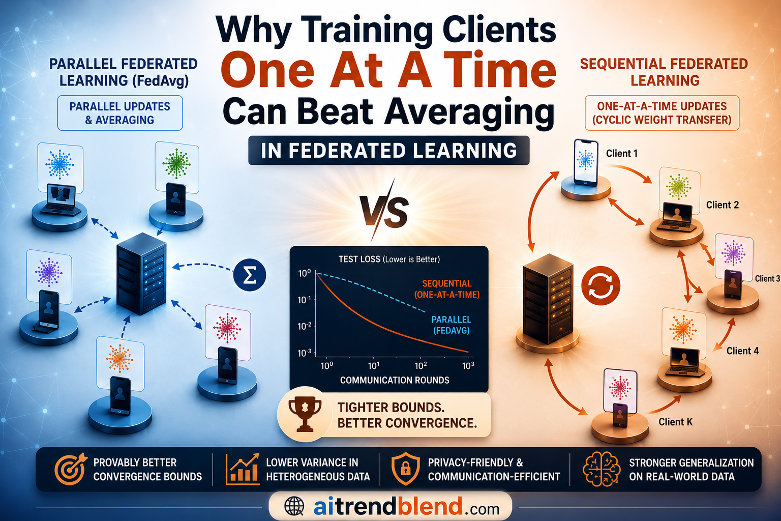
- The paper, by Yipeng Li and Xinchen Lyu of Beijing University of Posts and Telecommunications, proves the first matching upper and lower convergence bounds for sequential federated learning on data that differs from client to client.
- Sequential federated learning, where clients pass the model one after another instead of syncing through a server, gains an advantage of roughly one over the number of clients in its error terms compared with parallel averaging, under the standard heterogeneity assumption used across the field.
- The advantage shrinks or can even flip in the other direction only under a much stronger heterogeneity assumption, and only when the data is already close to identical across clients.
- Experiments on quadratic toy functions, logistic regression on LIBSVM data, and deep networks on Fashion MNIST, CIFAR 10, and CINIC 10 all back the theory.
- The result gives a concrete, testable reason to reconsider Cyclic Weight Transfer and Split Learning setups in medicine and other privacy sensitive fields rather than defaulting to FedAvg style averaging.
The core problem this paper is actually solving
Federated learning lets many devices or institutions train one shared model without shipping their raw data anywhere. Almost every popular recipe, from Google’s original FedAvg to Local SGD, follows the same parallel shape. Every client starts from the same global weights, runs a few steps of gradient descent locally, and sends the result back to a server that averages everyone’s update. That averaging step is doing real work. It is what keeps any single client’s idiosyncrasies from dragging the whole model off course.
There is a second family that gets far less attention, and this paper is squarely about it. In sequential federated learning, there is no central averaging moment at all. Client one trains on its own data for a fixed number of steps, then ships its updated weights directly to client two, who continues training from wherever client one left off, and so on until every client in the round has taken a turn. The final client’s output becomes the new global model for the next round. Cyclic Weight Transfer, used for years in multi institution medical imaging studies, works exactly this way, and so does the sequential variant of Split Learning at the network edge, where a neural network is physically divided between a resource constrained device and a server.
The appeal is practical. Nobody has to stand up and maintain a central parameter server, which is a real cost for a consortium of hospitals or a mesh of edge devices. There is no single point of failure sitting in the middle of the network, and communication happens client to client rather than funneling through one bottleneck. What has been missing, until this paper, is a rigorous answer to the question everyone quietly assumes they already know. Does training one client at a time actually converge as well as averaging them in parallel, especially once the clients hold genuinely different data.
Why prior work left this question open
The convergence theory of parallel federated learning is mature at this point. Researchers such as Xiang Li and coauthors, Ahmed Khaled and Peter Richtárik, Anastasia Koloskova and coauthors, and Sai Praneeth Karimireddy’s team behind SCAFFOLD have spent years pinning down exactly how heterogeneous client data slows FedAvg style training, and those results even spawned new algorithms designed to correct for it. Blake Woodworth and coauthors went further and proved matching lower bounds, showing those upper bounds were not just pessimistic guesses but the actual worst case.
Sequential federated learning never got the same treatment. A few recent papers, including work by Yae Jee Cho and coauthors and by Grigory Malinovsky and coauthors, studied federated learning with cyclic client participation, which overlaps with sequential training but does not fully cover the setup used in Cyclic Weight Transfer or sequential Split Learning. Li and Lyu’s own earlier conference paper, presented at NeurIPS 2023, established upper bounds for sequential federated learning. This new JMLR version is the extension, and the headline addition is the lower bound half of the story, the piece that lets anyone check whether an upper bound is actually tight or just a loose worst case estimate nobody has bothered to challenge.
There is also a structural reason sequential training is harder to analyze than it looks. In parallel training, one client’s local updates only depend on that client’s own randomness within the current round. In sequential training, client five’s updates depend on the randomness of clients one through four that already ran before it. And unlike SGD with random reshuffling, where you draw one data point per step, sequential federated learning runs many local optimization steps at each client before handing off, which stacks a second layer of complexity on top. The authors note that random reshuffling is technically a special case of their sequential setup, so their analysis has to generalize a well studied single step method into a multi step, multi client one.
How the two training recipes actually differ
It helps to see the update rules side by side in the paper’s own notation. Let M be the number of clients, K the number of local steps each client runs per round, and η the learning rate.
At the beginning of every round, sequential training draws a fresh random ordering of the clients rather than always visiting them in the same sequence, which matters for the analysis because it turns the process into something closer to a shuffled sampling scheme. The paper defines an effective learning rate \( \tilde{\eta} := \eta M K \) so that sequential and parallel training can be compared on genuinely equal footing, since one full round of sequential training moves the model through M times K total local steps before anyone averages anything.
Two ways to measure how different the clients are
The paper leans on a few standard assumptions about client heterogeneity that are worth understanding because the whole comparison hinges on which one you pick. Assumption 3 only bounds how far each client’s gradient sits from zero at the true optimum, which is a relatively forgiving condition. Assumption 4 is used for the non convex case and bounds the average squared distance between each client’s gradient and the global gradient everywhere, not just at the optimum. Assumption 5 is the strictest of the three, bounding the worst case client’s deviation from the global gradient at every point in the parameter space. As the authors put it plainly, if every client’s objective is identical there is no heterogeneity and all of these constants collapse to zero, but the reverse is not automatically true, since these assumptions only capture first order behavior.
The bounds themselves, and what they say
Theorem 3 in the paper gives upper bounds on how close sequential federated learning gets to the optimal solution after R training rounds, split into three regimes depending on whether the local objective functions are strongly convex, generally convex, or non convex. Each bound is built from two pieces that pull in opposite directions, an optimization term that shrinks as training runs longer, and an error term driven by both the noise in stochastic gradients and the heterogeneity across clients. Picking too large a learning rate makes the optimization term vanish faster but inflates the error term, so Corollary 4 works out the learning rate schedule that balances the two.
The part worth staring at is the heterogeneity term, the one containing \( \zeta_*^2 \), which shrinks proportionally to M. That single factor of M in the denominator is the mathematical fingerprint of the paper’s central claim. When the corresponding bound is worked out for parallel federated learning in Theorem 7, the matching heterogeneity term does not carry that extra M at all. Under Assumption 3, sequential training’s error terms come out smaller by a factor of the number of clients, and the same relationship holds for the general convex case and, under Assumption 4, for the non convex case without exception.
The lower bound construction is genuinely careful work, built across two separate appendices, one isolating the stochastic noise contribution and one isolating the heterogeneity contribution, using techniques adapted from Woodworth’s minibatch versus local SGD paper, Chulhee Yun’s shuffling analysis, and Jaeyoung Cha’s tighter shuffling bounds. The authors even check their sequential federated learning bounds against the best known bounds for plain SGD with random reshuffling, since reshuffled SGD is the special case where each client runs exactly one local step. The general convex and non convex rates match the reshuffling literature exactly. In the strongly convex case, reshuffled SGD keeps a small edge on its optimization term thanks to a technique called Shuffling Variance that the authors note as an open direction for extending to the federated setting.
Where the advantage disappears
The honest part of this paper, and the part that keeps it from reading like a sales pitch for sequential training, is Section 5.2. Under the stricter Assumption 5, where the worst client’s gradient deviation is bounded everywhere rather than just at the optimum, the authors compare their results against Woodworth’s parallel federated learning bounds and find a genuine tradeoff. Parallel training’s optimization term decays faster in this regime, while sequential training still wins on the error terms. Work out the arithmetic and there is a narrow condition, roughly when the heterogeneity constant is extremely small relative to the number of training rounds, where parallel averaging pulls ahead. Push the heterogeneity back up even slightly and sequential training regains the lead.
The practical reading is straightforward. If client data across your federation is nearly identical already, the choice between sequential and parallel training barely matters and parallel training may have a small edge. The moment real world heterogeneity shows up, which is the normal case for hospitals, phones, or edge devices with genuinely different populations, sequential training’s advantage reasserts itself.
What the experiments actually show
Theory is only convincing when it survives contact with real training runs, and the authors ran three separate experiments of increasing realism.
Quadratic toy functions
The simplest test uses one dimensional quadratic objectives split across two clients, with the learning rate for sequential training deliberately set to half that of parallel training as the theory recommends. Across ten groups of functions with increasing heterogeneity in both the gradients and the curvature, sequential training beat parallel training in every group except the two where the clients had zero heterogeneity in curvature, which the authors attribute honestly to a gap in the theory itself. The existing assumptions do not fully capture second order Hessian information, something Kumar Kshitij Patel and coauthors have also flagged as an open problem in the wider local SGD literature.
Logistic regression on real tabular data
Moving to a more realistic setup, the team trained logistic regression classifiers on the a9a and w8a datasets from the LIBSVM library, split across 1000 simulated clients using an Extended Dirichlet partitioning strategy where each client only sees samples from one or two class labels. With only one label per client, the most extreme heterogeneity setting, sequential training clearly outperformed parallel training on training loss. With two labels per client, the gap narrowed until the two methods tracked each other closely, exactly the pattern the theory predicts.
Deep networks on image data
The most convincing test trains a CNN on Fashion MNIST and a VGG 9 network on CIFAR 10 and CINIC 10, splitting each dataset across 500 to 1000 clients with the same Dirichlet style partitioning at three heterogeneity levels. The results are summarized below using the paper’s own reported top one test accuracy after the last 100 training rounds, averaged across three random seeds.
| Dataset | Method | C = 1 test | C = 2 test | C = 5 test |
|---|---|---|---|---|
| Fashion MNIST | Parallel | 85.77 | 88.55 | 90.70 |
| Fashion MNIST | Sequential | 87.60 | 89.66 | 90.92 |
| CIFAR 10 | Parallel | 73.84 | 78.99 | 83.47 |
| CIFAR 10 | Sequential | 81.05 | 83.34 | 84.73 |
| CINIC 10 | Parallel | 52.27 | 61.96 | 68.45 |
| CINIC 10 | Sequential | 61.52 | 67.31 | 70.82 |
C is the number of class labels each simulated client is allowed to see, so smaller C means a client’s local data looks less and less like the overall population. The gap between sequential and parallel training is largest on CIFAR 10 at the harshest heterogeneity setting, over seven points of test accuracy, and it compresses toward almost nothing once every client sees five classes worth of data. That shrinking gap as heterogeneity falls is precisely the signature the convergence bounds predicted before a single experiment was run.
Why this matters beyond the benchmark tables
The most direct beneficiaries of this result are exactly the communities that already use sequential training out of necessity rather than by theoretical choice. Multi institution medical imaging consortiums using Cyclic Weight Transfer, as documented in Ken Chang and coauthors’ work on distributed deep learning across hospitals, have been running something close to sequential federated learning for years without a convergence theory to justify it under real data heterogeneity, which in medical imaging is often severe given how differently scanners, patient populations, and protocols vary between sites. Split Learning deployments at the network edge, where a full model gets divided between constrained devices and a server, use a sequential training pattern for exactly the reason this paper studies, and the authors note their theory transfers directly to that setting.
There is also a broader lesson for anyone designing a new federated system from scratch. The instinct to reach for FedAvg style parallel averaging is understandable given how dominant it is in tutorials and libraries, but this paper is a reminder that the peer to peer, no central server alternative is not a compromise made purely for infrastructure convenience. Under the heterogeneity conditions federated learning was invented to handle in the first place, sequential training can be the mathematically stronger choice, not just the operationally simpler one.
Honest limitations of the paper
A few things keep this from being the final word on the topic, and the authors say so themselves in the conclusion. The lower bounds for the non convex case are still missing entirely, for both sequential federated learning and for reshuffled SGD more generally, so the strongest claim in the paper, that sequential training beats parallel training without exception in the non convex setting, currently rests on an upper bound comparison alone rather than a matched lower bound. The lower bounds that do exist are also described by the authors as loose for small numbers of training rounds, only becoming tight asymptotically as R grows.
The unexpected results in the quadratic experiment, where parallel training tied or beat sequential training when clients had identical curvature, point to a real gap in the underlying assumptions, which only capture first order gradient information and do not fully account for second order Hessian differences between clients. The authors flag this explicitly rather than papering over it, and they note that Jianyu Wang and coauthors have separately argued that these standard heterogeneity assumptions can underestimate what parallel averaging is actually capable of once the aggregation step’s own smoothing effect is accounted for. Finally, every experiment here uses simulated heterogeneity through Dirichlet style partitioning of standard benchmark datasets, which is the field’s normal practice but is still a simplification of how heterogeneous real deployments across hospitals, phones, or IoT sensors actually look.
Complete PyTorch implementation of sequential and parallel federated learning
The code below is a compact, runnable reimplementation of Algorithm 1 and Algorithm 2 from the paper. It trains a small classifier under both training schemes on synthetic heterogeneous data so you can see the accuracy gap the paper describes appear on your own machine. It includes a smoke test on dummy data at the end so you can confirm it runs before pointing it at a real dataset.
Running this on a laptop should print two lists of rising accuracy numbers followed by a pass message. If you raise the heterogeneity argument and rerun both methods with the same seed, you should see the sequential run pull ahead of the parallel run more often than not, which is the same pattern reported in the paper’s own quadratic and logistic regression experiments, though a tiny synthetic MLP will never reproduce the exact numbers from a VGG 9 run on CIFAR 10.
Where this leaves the field
Federated learning research has spent most of its energy on the parallel branch of the family tree, in large part because FedAvg got there first and because industry deployments with millions of phones genuinely need the parallelism. This paper is a useful correction to that emphasis. It does not claim sequential training is universally better, and it is careful to mark the narrow regime where parallel training keeps an edge. What it does establish, with both directions of the bound rather than just a hopeful upper limit, is that the peer to peer alternative already used informally in medical imaging and edge Split Learning has real theoretical backing precisely in the messy, heterogeneous conditions those fields actually operate under.
The conceptual shift worth remembering is that sequential training is not simply parallel training done inefficiently one client at a time. The order in which clients are visited, combined with the fact that each round samples a fresh random permutation, gives sequential federated learning some of the same variance reducing properties that make random reshuffling a stronger optimizer than plain stochastic gradient descent with replacement. That connection to a decades old idea in stochastic optimization is what lets the authors borrow proof techniques from the shuffling literature rather than building an analysis from nothing.
Where this could travel next is fairly clear from the authors’ own closing questions. They flag the missing non convex lower bound as an open problem, they wonder whether extrapolation techniques already shown to speed up parallel federated learning could be adapted to the sequential setting, and they point at Hessian level heterogeneity as the likely explanation for the handful of experimental cases where their theory did not predict the winner correctly. Any of those three would be a natural follow up paper, and none of them would require throwing out the framework built here.
For practitioners the takeaway is more immediate than any of that. If your federation already looks sequential, whether that is a hospital consortium doing Cyclic Weight Transfer or an edge deployment doing Split Learning, this paper gives you a reason to stop treating that as a compromise forced by infrastructure and start treating it as a training scheme with its own, now proven, statistical advantages under exactly the kind of data heterogeneity that made federated learning necessary in the first place.
None of this argues for abandoning parallel federated learning, which still wins on wall clock time and remains the right default when a system genuinely needs every client’s compute running at once. What changes after reading this paper is the default assumption. Sequential training is not the fallback option for teams that could not afford a central server. Under heterogeneous data, the more common situation in practice than the tidy identically distributed case textbooks like to assume, it can be the mathematically stronger choice on its own terms.
Read the source material
The full paper, including every proof referenced above, is published in JMLR 26 and available as arXiv:2311.03154.
Frequently asked questions
What is the difference between sequential and parallel federated learning
Parallel federated learning has every client train from the same starting weights at the same time and then averages their results on a central server, the pattern behind FedAvg. Sequential federated learning has clients train one after another, each one continuing from the previous client’s final weights, with no central averaging step and no requirement for a central server at all.
Does sequential federated learning really beat parallel federated learning
Under the standard heterogeneity assumption used across the federated learning literature, the paper proves sequential training’s error terms are smaller by a factor equal to the number of clients, and confirms this with matching lower bounds and with experiments on quadratic functions, logistic regression, and deep networks. The advantage narrows and can occasionally reverse only under a stricter heterogeneity assumption and only when client data is already close to identical.
Is sequential federated learning slower in practice
Yes, in wall clock terms. Because each client has to wait for the previous one to finish, a single round of sequential training with M clients takes roughly M times longer than a round of parallel training, even though it often reaches a better model per round on heterogeneous data. Choosing between them means weighing training quality against latency for your specific deployment.
What is Cyclic Weight Transfer and how does it relate to this paper
Cyclic Weight Transfer is a training method used in multi institution medical imaging research where a model is passed from hospital to hospital in sequence, each one training on its own patient data before passing the model along. It is a real world example of sequential federated learning, and this paper’s convergence bounds apply directly to it.
Why does data heterogeneity matter so much for this comparison
When every client’s data looks statistically similar, both training methods converge to roughly the same place and the choice between them matters less. Real deployments across hospitals, phones, or sensors almost never look like that, and the paper shows sequential training’s mathematical advantage over parallel training grows specifically as that heterogeneity increases.
Where can I see the code used in the paper’s experiments
The authors released their experiment code publicly, linked in the paper and in the CTA box above, alongside the compact PyTorch reimplementation included in this article that you can run yourself on synthetic heterogeneous data.
Limitations
This article summarizes claims and numbers exactly as reported in the source paper. The non convex lower bound gap, the loose small round behavior of the existing lower bounds, and the unexplained quadratic experiment cases are all limitations the original authors state themselves rather than issues found independently by this analysis. Readers building a production federated system should treat the specific numeric results in the tables above as reported under the paper’s exact experimental settings, including its particular Dirichlet partitioning scheme and network architectures, rather than as guarantees that will transfer unchanged to a different dataset or model family.
This analysis is based on the published paper and an independent evaluation of its claims.