
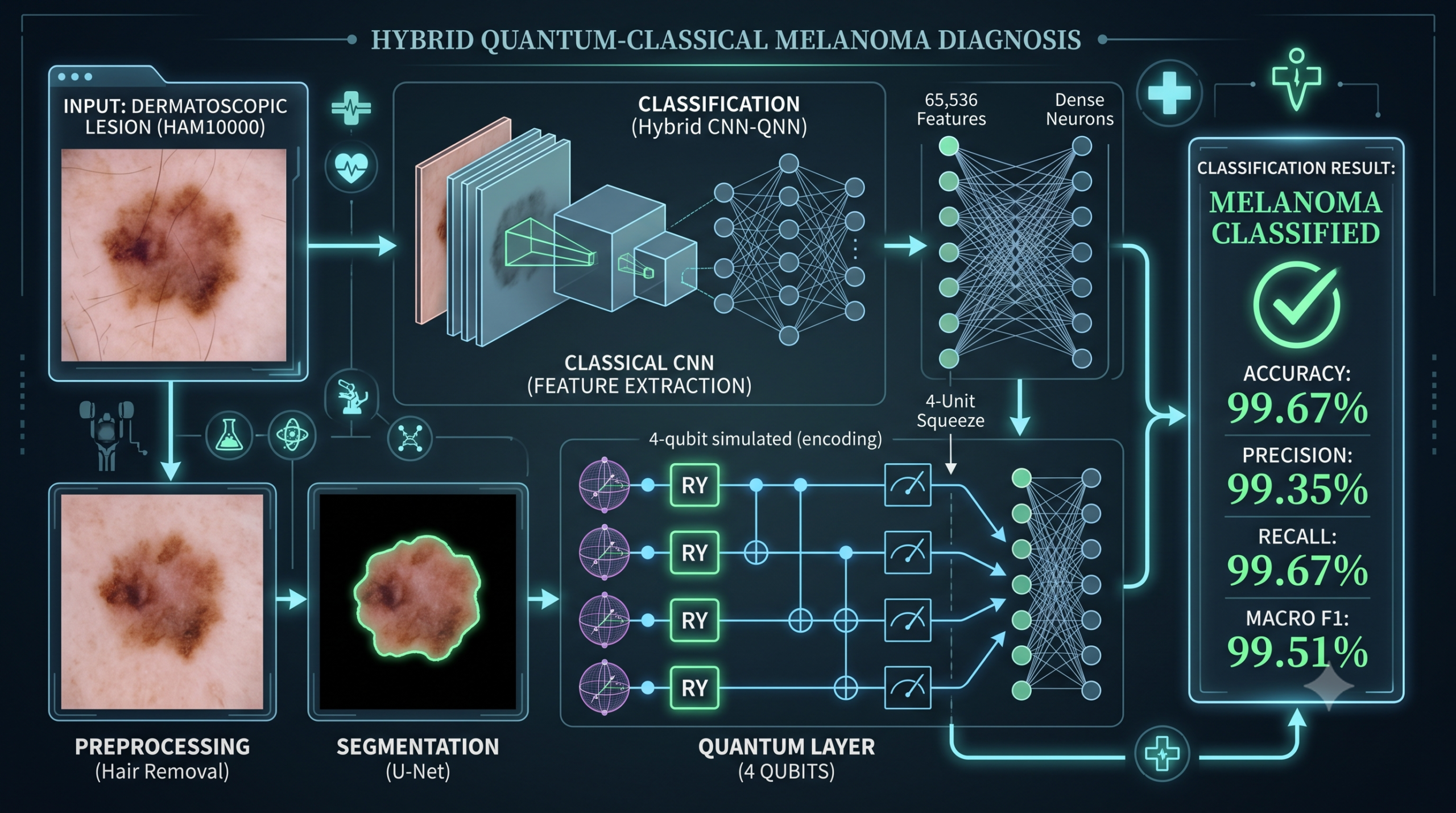
A patient sits under a dermatoscope while a clinician tries to decide, in under a minute, whether an irregular brown patch on their shoulder is an ordinary mole or something that needs a biopsy. That judgment call happens millions of times a year, and it is exactly the gap a new paper from researchers at the University of Milan, the European Institute of Oncology, and SKEMA Business School is trying to close. Their tool pairs an ordinary convolutional network with a four qubit quantum circuit, runs it on the public HAM10000 dermatoscopic image set for Melanoma Classification, and reports accuracy above 99 percent. That number is real. What it actually measures is more complicated than the headline suggests.
Key points
- The study builds a full pipeline for melanoma detection covering hair removal, lesion segmentation with U-Net, and classification with a hybrid CNN and quantum neural network called CNN-QNN.
- On the HAM10000 dataset the hybrid model reports 99.67 percent accuracy, 99.35 percent precision, 99.67 percent recall, and a macro F1 score of 99.5 percent.
- The quantum component is a simulated four qubit circuit, not real quantum hardware, and it receives only four numbers per image after the CNN has already compressed a large feature map down to that size.
- The paper never trains a classical only version of the exact same pipeline for direct comparison, so how much of the 99.67 percent comes from the quantum layer specifically is not established by the reported experiments.
- All testing used k fold cross validation on the same single dataset with no external clinical cohort, and the authors are candid that generalization to real hospital settings remains unproven.
- This article explains what the research measured, walks through the architecture and math, and flags the gaps a careful reader should weigh before treating this as a clinical breakthrough.
Read this first
This article explains a piece of published research. It is not medical advice, it is not a diagnostic tool, and it should not be used to evaluate a real skin lesion. If you or someone you know has a mole or skin mark that looks irregular, changes shape, bleeds, or otherwise concerns you, see a dermatologist or qualified physician. Nothing in this piece substitutes for a clinical exam.
Why melanoma detection keeps drawing AI researchers back
Melanoma is not the most common skin cancer, but it is the one that kills. It starts in melanocytes, the pigment producing cells in the skin, and its incidence in fair skinned populations has climbed by roughly 3 to 5 percent a year since the middle of the twentieth century, according to the figures the authors cite. Depending on the population, that works out to somewhere between 20 and 60 new cases per 100,000 people annually. Caught early, melanoma is usually treatable. Caught late, after it has moved past the surface layers of the skin, survival drops sharply.
The standard screening tool is still a dermatologist’s trained eye, sometimes helped by a dermatoscope, applying the familiar ABCDE checklist. A mole gets flagged when it shows asymmetry, an irregular border, more than one color, a diameter over 6 millimeters, or visible change over time. That heuristic works well in the hands of an experienced specialist, but it is still a judgment call, and judgment calls vary between clinicians and get harder when a lesion is early or only partially typical. That variability is the opening computer aided diagnosis keeps trying to fill, and it is why nearly every recent melanoma paper, this one included, frames its contribution around reducing subjectivity and catching cases earlier.
What the paper actually built
The authors, Maria Frasca, Ilaria Cutica, Gabriella Pravettoni, and Davide La Torre, structured their system as three stages that run in sequence. First comes preprocessing, which strips noise and body hair out of the raw dermatoscopic photo. Second comes segmentation, which isolates the lesion from the surrounding skin. Third comes classification, where the hybrid CNN-QNN model decides what kind of lesion it is looking at.
Cleaning up the image before anything else happens
Dermatoscopic photos are notoriously messy. Body hair crosses right over the lesion, lighting varies from shot to shot, and sensor noise adds texture that has nothing to do with the skin. The team applied a Gaussian filter first, a standard smoothing pass that softens high frequency noise while trying not to blur the lesion’s actual edges. Then, because hair removal is its own small research problem, they tested two separate approaches. One used the Canny edge detector to trace hair strands, closed the gaps with morphological operations, and filled the resulting gaps with a coherence based inpainting technique, later enhanced with a GAN based inpainting model trained on dermoscopic images. The other trained a dedicated autoencoder, a compact encoder and decoder network with skip connections, to learn what a hairless version of the same lesion should look like and reconstruct it directly.
Both hair removal methods eventually feed into the same segmentation and classification steps, and the paper reports results for each path separately, which turns out to matter a great deal once you get to the numbers.
Finding the lesion boundary
Once the hair is gone, the pipeline needs to know exactly where the lesion is. The authors tried two techniques here as well. Otsu’s method is a classic global thresholding algorithm that finds a single brightness cutoff separating lesion from skin. It is fast and simple, but it struggles with uneven lighting and lesions that blend gradually into surrounding skin. The second approach is a U-Net, a convolutional encoder decoder network with skip connections that has become close to a default choice for medical image segmentation since its original description. The U-Net in this paper follows the classic four level contracting and four level expanding structure, doubling channels on the way down and halving them on the way back up, with each expansion stage concatenating features from the matching contraction stage. Images were resized to 128 by 128 pixels, brightness boosted by a factor of 1.5, and the network trained for 100 epochs with the Adam optimizer using binary crossentropy loss.
The classifier where the quantum computing happens
This is where the paper’s central claim lives. The classifier takes the segmented lesion image, resized again to 128 by 128 pixels and converted to grayscale, and runs it through three convolutional layers with 16, 32, and 64 filters respectively, each followed where appropriate by 2 by 2 max pooling. That produces a feature map that gets flattened into a vector of size 64 times 32 times 32, which works out to 65,536 numbers. A fully connected layer, FC1, compresses that entire vector down to just four values, one for each of the four simulated qubits the model uses.
Those four numbers get mapped onto rotation angles and fed into a simulated quantum circuit. Each qubit receives a rotation around the Y axis based on its assigned value, CNOT gates entangle the qubits with each other, and the circuit is measured along the Z axis to produce four output values. Those four numbers pass through another fully connected layer, FC2, expanding them to 128 units, and a final layer, FC3, maps that to the number of output classes using softmax. The whole thing trains end to end with the Adam optimizer at a learning rate of 0.001, chosen after testing 0.01, 0.001, and 0.0001 against each other, using cross entropy loss and five fold cross validation.
Because the paper is explicit that a genuine quantum neural network requires actual quantum hardware, everything here ran as a classical simulation on a workstation with an Intel Core i9-10885H processor and an NVIDIA Quadro RTX 3000 GPU. That detail matters for the limitations section below, and it is worth holding onto now.
The math behind the quantum layer
A classical neuron applies an activation function to a weighted sum of its inputs plus a bias term.
Classical neuron output
\[ \text{Output} = \text{Activation}\left(\sum_i w_i x_i + b\right) \]A quantum neuron instead applies a parameterized quantum gate to an input quantum state.
Quantum state transformation
\[ |\psi_{out}\rangle = U(\theta)|\psi_{in}\rangle \]In this paper’s circuit, the gate that does most of the work is a rotation around the Y axis, parameterized by an angle theta derived from the CNN’s compressed feature vector.
RY rotation gate
\[ R_Y(\theta) = \begin{bmatrix} \cos(\theta/2) & -\sin(\theta/2) \\ \sin(\theta/2) & \cos(\theta/2) \end{bmatrix} \]Entanglement between qubit pairs comes from a CNOT gate, which flips a target qubit’s state conditioned on a control qubit.
CNOT gate matrix
\[ \text{CNOT} = \begin{bmatrix} 1 & 0 & 0 & 0 \\ 0 & 1 & 0 & 0 \\ 0 & 0 & 0 & 1 \\ 0 & 0 & 1 & 0 \end{bmatrix} \]After the RY rotations and CNOT entanglement have been applied across all four qubits, each qubit is measured along the Z axis, and those four expectation values become the input to the rest of the classifier. Training the angles theta happens the same way any neural network parameter gets trained, by nudging them against the gradient of the loss function, except that quantum circuits typically need the parameter shift rule rather than ordinary backpropagation to compute that gradient, since the circuit itself is not directly differentiable the way a matrix multiplication is.
What the results actually show
The headline numbers come from the combination of U-Net segmentation, autoencoder based hair removal, and the CNN-QNN classifier. On that configuration the model reports 99.67 percent accuracy, 99.35 percent precision, 99.67 percent recall, a macro F1 score of 99.51 percent, and an AUC of 99.76 percent. The Canny algorithm hair removal path performs slightly worse but still strong, landing at 98.37 percent accuracy with U-Net segmentation.
The tables below reproduce the paper’s reported numbers exactly.
| Metric | Original dataset | Otsu segmentation | U-Net segmentation |
|---|---|---|---|
| Accuracy | 73.09% | 73.09% | 78.07% |
| Precision | 53.42% | 53.42% | 73.14% |
| Recall | 73.09% | 73.09% | 78.07% |
| F1 score | 61.72% | 61.72% | 73.46% |
| AUC | 48.57% | 42.17% | 85.64% |
| Metric | Original dataset | Otsu segmentation | U-Net segmentation |
|---|---|---|---|
| Accuracy | 73.09% | 73.09% | 99.67% |
| Precision | 53.42% | 53.42% | 99.35% |
| Recall | 73.09% | 73.09% | 99.67% |
| F1 score | 61.72% | 61.72% | 99.51% |
| AUC | 52.97% | 63.87% | 99.76% |
| Study | Accuracy | Precision | Recall |
|---|---|---|---|
| Adegun et al 2019 | 90% | — | — |
| Seeja et al | 92% | 91% | 90% |
| Daghrir et al 2020 | 95% | 93% | 92% |
| Acosta et al 2021 | 92% | 91% | 90% |
| Sivakumar et al 2024 | 93% | 91% | 90% |
| Lopez et al 2023 | 94% | — | — |
| Li et al 2022 | 95% | — | — |
| Razmjooy et al 2020 | 95% | — | — |
| Cirrincione et al 2023 | 96% | — | — |
| Proposed CNN-QNN | 99.67% | 99.35% | 99.67% |
Notice the jump between Table 1 and Table 2. With no hair removal at all, U-Net segmentation only gets accuracy to 78.07 percent. Add the autoencoder based hair removal step to the exact same U-Net segmentation and classifier, and accuracy jumps to 99.67 percent. That is a 21 point swing driven entirely by preprocessing, using the identical CNN-QNN classifier in both rows. It is a genuinely useful finding about the value of careful preprocessing on this dataset. It also means the preprocessing pipeline, not the quantum layer, explains most of the distance between this paper’s headline number and the 90 to 96 percent range the comparison studies in Table 5 report.
Takeaway
The largest single jump in reported accuracy across the whole study comes from swapping in autoencoder based hair removal before segmentation, not from anything involving qubits. That is worth remembering every time the 99.67 percent figure gets quoted on its own.
The paper also runs a comparison against a ResNet-50 classifier using the exact same preprocessing and segmentation pipeline, and looks at the two models through principal component analysis. The explained variance in the first two principal components is almost identical between the two models, 6.3778 percent for ResNet-50 against 6.3992 percent for CNN-QNN. The intra class distance, meaning how spread out feature representations are within the same lesion category, comes out slightly lower for CNN-QNN at 9.802606 against 9.960223 for ResNet-50. The inter class distance, meaning how far apart benign and melanoma clusters sit from each other, is very slightly lower for CNN-QNN too, 9.931106 against 9.980202. The authors themselves describe this difference as not substantial, and they flag that a smaller intra class distance can actually be a sign of overfitting rather than a sign of better generalization, a caveat that is easy to miss if you only read the abstract.
Where the analysis gets more interesting than the abstract lets on
A four number bottleneck is doing the quantum part of the work
Here is the detail that changes how you should read the 99.67 percent figure. The convolutional stack produces a feature map that flattens to 65,536 values. Before any quantum operation happens, a single fully connected layer squeezes that down to exactly four numbers, one per qubit. Whatever information the quantum circuit works with, it works with only those four compressed values, not the rich feature map the CNN produced. After the quantum circuit measures its four qubits, another fully connected layer expands those four numbers back out to 128 units before the final classification layer.
That architecture puts almost the entire representational load on the classical convolutional layers and the two surrounding fully connected layers. The quantum circuit sits in the middle as a four dimensional transformation, RY rotations followed by CNOT entanglement, applied to whatever the CNN already decided mattered. It is a real component and it does contribute some nonlinearity that a purely linear layer would not, but calling the resulting system a quantum classifier somewhat overstates how much of the decision making the quantum piece is actually doing versus how much sits in the surrounding classical layers.
The paper never isolates the quantum layer’s actual contribution
The introduction explicitly promises, as one of the paper’s four contributions, a detailed analysis of the impact of the quantum layer through ablation studies showcasing its role in boosting classification performance. Reading through Section 7, that specific ablation does not appear. What the results section actually contains is a comparison between the full CNN-QNN pipeline and a separately trained ResNet-50 model, which differs from CNN-QNN in far more ways than just the presence or absence of a quantum layer. ResNet-50 has a completely different convolutional architecture, different depth, and different parameter count. A true ablation would take the exact CNN-QNN architecture described in Section 6.3, remove only the quantum circuit, replace it with an ordinary four unit dense layer or a small nonlinear block of comparable size, and retrain that variant on the identical preprocessing and segmentation pipeline. That specific experiment is not in the paper as published. Without it, the claim that the quantum layer specifically drives the accuracy gain over conventional CNNs is plausible but not demonstrated by the evidence presented.
The promised statistical significance testing is also missing
Contribution four in the introduction promises an exploration of statistical significance in the experimental results to ensure robustness and reliability. The results section reports point estimates for accuracy, precision, recall, F1, and AUC, along with the PCA distance comparisons, but no confidence intervals, no p values, and no significance test comparing CNN-QNN against ResNet-50 or against the other studies in Table 5 appear anywhere in the paper. The five fold cross validation the authors describe using would have been a natural source for computing a standard deviation or a confidence interval across folds, but those numbers are not reported. That is a meaningful gap between what the introduction promises and what the results section delivers, and it means the difference between 99.67 percent and, say, 96 percent from a competing paper on a different dataset and protocol should be read as a difference in reported point estimates rather than a statistically established improvement.
Table 5 compares apples to a fairly different set of fruit
Every row in Table 5 comes from a separate study with its own dataset split, its own preprocessing choices, and in several cases a different dataset entirely. Some of the comparison studies use Mask R-CNN and ResNet152, others use SVM and Random Forest on top of CNN features, and others rely on Transformer architectures. None of them were rerun on the exact same train and test split as the CNN-QNN model in this paper. That is a common practice across the melanoma classification literature, not a flaw unique to this paper, but it does mean the ranking in Table 5 tells you which numbers got published, not which method would actually win in a head to head test on identical data.
The authors’ own caveat, that the intra class distance difference between ResNet and CNN-QNN is not substantial, is the most honest sentence in the results section, and it is worth reading twice. Frasca, Cutica, Pravettoni, and La Torre, Intelligence Based Medicine, 2025
Class imbalance is handled but not fully neutralized
HAM10000 is heavily skewed toward benign melanocytic nevi, with 6,705 nevus images against 1,113 melanoma images and 1,099 benign keratosis like lesions, out of roughly 10,000 total. The authors chose not to rebalance the dataset, reasoning that the natural imbalance reflects real clinical prevalence, and instead applied a loss function weighting scheme that penalizes errors on minority classes more heavily. That is a defensible design choice and the paper reports macro averaged metrics, which treat every class equally regardless of how many examples it has, rather than a simple overall accuracy that a majority class predictor could inflate. Still, weighting the loss function is not the same as validating performance on an external, differently distributed population, and the paper is explicit that this remains untested.
Takeaway
Macro averaged metrics and loss weighting are reasonable mitigations for class imbalance, but they were validated only through cross validation on the same HAM10000 images the model trained on, not on an independent cohort with a different case mix.
The clinical translation gap
A benchmark number on a public dataset and a tool a dermatologist could actually rely on in clinic are two different things, and this paper is candid about the distance between them. Three gaps stand out. First, everything ran through k fold cross validation on HAM10000 alone. No external test set from a different clinic, a different camera, or a different patient population was used, so it is not yet known how the model performs when the imaging conditions change even modestly. Second, the quantum component only exists as a classical simulation. Real quantum hardware was not used anywhere in this study, and the authors state directly that simulating quantum circuits becomes exponentially more demanding as qubit count grows, which caps how much larger or more expressive the quantum layer could get without dramatically higher compute cost. Third, HAM10000 itself, useful as it is, was assembled from a specific set of clinical sources and does not represent the full diversity of skin tones, lesion presentations, and imaging equipment a deployed tool would encounter worldwide. None of these gaps make the research uninteresting. They do mean the 99.67 percent figure describes performance on a benchmark, not performance you should expect in a dermatology clinic tomorrow.
Honest limitations
Beyond the analytical gaps above, the paper’s own discussion section names several constraints worth repeating in plain terms. The quantum layer requires simulating qubits on classical hardware because real quantum computers remain largely inaccessible, and that simulation grows exponentially more expensive as the number of qubits increases, which limits how far this exact approach could scale to larger images or richer quantum layers. Training a quantum circuit also does not use ordinary backpropagation the way the rest of the network does, so integrating the classical CNN with the quantum layer required the parameter shift rule and added engineering complexity the paper acknowledges as nontrivial. The entire evaluation lives on one dataset, HAM10000, split only through cross validation rather than tested on a genuinely separate clinical cohort, so claims about generalization outside that dataset remain open. Finally, the hardware used to run these experiments, a single mobile workstation with a Quadro RTX 3000 GPU, is modest by research standards, and the authors note that even at that scale the addition of quantum layers meaningfully increased training time and memory use compared to a purely classical network.
The PyTorch implementation
The code below reconstructs the hybrid CNN and quantum neural network architecture described in Section 6.3 of the paper. The quantum circuit is implemented as an explicit four qubit statevector simulation using pure PyTorch tensors, applying RY rotation gates followed by a ring of CNOT gates, then measuring the Pauli Z expectation value of each qubit, which mirrors the RY encoding, CNOT entanglement, and Z axis measurement the paper describes. It includes the full model class, the training loop, an evaluation function using the macro averaged metrics the paper reports, and a runnable smoke test on random dummy data so you can confirm the whole pipeline executes correctly before pointing it at real dermatoscopic images.
import torch
import torch.nn as nn
import torch.nn.functional as F
from torch.utils.data import DataLoader, TensorDataset
import math

# ---------------------------------------------------------------------
# Simulated quantum circuit
# Reproduces the RY encoding, CNOT entanglement ring, and Pauli Z
# measurement described in Section 6.3 of the paper, using an explicit
# statevector simulation so the whole model stays differentiable in
# plain PyTorch with no external quantum computing library required.
# ---------------------------------------------------------------------

class QuantumCircuitSimulator(nn.Module):
    def __init__(self, n_qubits=4):
        super().__init__()
        self.n_qubits = n_qubits
        self.dim = 2 ** n_qubits
        # Trainable rotation weights applied after the data encoding,
        # matching the paper's randomly initialized q_params that are
        # optimized during training.
        self.q_params = nn.Parameter(torch.randn(n_qubits) * 0.1)

    def _ry_matrix(self, theta):
        # Builds the 2 by 2 RY rotation matrix from Equation 9 in the paper.
        cos = torch.cos(theta / 2)
        sin = torch.sin(theta / 2)
        return torch.stack([
            torch.stack([cos, -sin]),
            torch.stack([sin, cos])
        ])

    def _apply_single_qubit_gate(self, state, gate, qubit_idx, batch_size):
        # Applies a single qubit gate to the full statevector by reshaping
        # the state so the target qubit's axis is isolated, contracting
        # with the gate, then restoring the original shape.
        shape = [batch_size] + [2] * self.n_qubits
        state = state.view(*shape)
        state = torch.movedim(state, qubit_idx + 1, -1)
        flat_shape = state.shape
        state = state.reshape(-1, 2)
        state = state @ gate.T
        state = state.reshape(flat_shape)
        state = torch.movedim(state, -1, qubit_idx + 1)
        return state.reshape(batch_size, -1)

    def _apply_cnot(self, state, control, target, batch_size):
        # Applies a CNOT gate by flipping the target qubit only in the
        # slice of the statevector where the control qubit is one,
        # matching the matrix in Equation 10 of the paper.
        shape = [batch_size] + [2] * self.n_qubits
        state = state.view(*shape)
        state = torch.movedim(state, control + 1, 1)
        state = torch.movedim(state, target + 1 if target < control else target, 2)
        on_branch = state[:, 1].clone()
        state[:, 1] = torch.flip(on_branch, dims=[1])
        state = torch.movedim(state, 2, target + 1 if target < control else target)
        state = torch.movedim(state, 1, control + 1)
        return state.reshape(batch_size, -1)

    def forward(self, x):
        # x has shape (batch, n_qubits) and holds the values FC1 produced.
        batch_size = x.shape[0]
        state = torch.zeros(batch_size, self.dim, dtype=torch.float32, device=x.device)
        state[:, 0] = 1.0

        # RY encoding, one rotation per qubit driven by the CNN feature
        # value plus a trainable offset.
        for q in range(self.n_qubits):
            theta = x[:, q] + self.q_params[q]
            for b in range(batch_size):
                gate = self._ry_matrix(theta[b])
                single = self._apply_single_qubit_gate(
                    state[b:b+1], gate, q, 1
                )
                state = state.clone()
                state[b:b+1] = single

        # Ring of CNOT gates entangling neighboring qubits, matching the
        # entanglement step described after Equation 10.
        for q in range(self.n_qubits):
            control, target = q, (q + 1) % self.n_qubits
            state = self._apply_cnot(state, control, target, batch_size)

        # Pauli Z expectation per qubit, the classical readout the paper
        # describes passing into the dense layers that follow.
        probs = state ** 2
        expectations = []
        shape = [batch_size] + [2] * self.n_qubits
        probs_reshaped = probs.view(*shape)
        for q in range(self.n_qubits):
            axes = [i for i in range(1, self.n_qubits + 1) if i != q + 1]
            marginal = probs_reshaped.sum(dim=axes)
            expectation = marginal[:, 0] - marginal[:, 1]
            expectations.append(expectation)
        return torch.stack(expectations, dim=1)


# ---------------------------------------------------------------------
# Hybrid CNN plus QNN classifier
# Mirrors the three convolutional layers, the FC1 to n_qubits bridge,
# the quantum layer, and the FC2 and FC3 output layers from Section 6.3.
# ---------------------------------------------------------------------

class CNNQNNHybrid(nn.Module):
    def __init__(self, n_classes=7, n_qubits=4, image_size=128):
        super().__init__()
        self.conv1 = nn.Conv2d(1, 16, kernel_size=3, stride=1, padding=1)
        self.conv2 = nn.Conv2d(16, 32, kernel_size=3, stride=1, padding=1)
        self.conv3 = nn.Conv2d(32, 64, kernel_size=3, stride=1, padding=1)
        self.pool = nn.MaxPool2d(2, 2)

        pooled_size = image_size // 4  # two pooling steps, after conv2 and conv3
        flat_dim = 64 * pooled_size * pooled_size

        self.fc1 = nn.Linear(flat_dim, n_qubits)
        self.quantum_layer = QuantumCircuitSimulator(n_qubits=n_qubits)
        self.fc2 = nn.Linear(n_qubits, 128)
        self.fc3 = nn.Linear(128, n_classes)

    def forward(self, x):
        x = F.relu(self.conv1(x))
        x = F.relu(self.conv2(x))
        x = self.pool(x)
        x = F.relu(self.conv3(x))
        x = self.pool(x)
        x = x.view(x.size(0), -1)
        x = torch.tanh(self.fc1(x)) * math.pi
        x = self.quantum_layer(x)
        x = F.relu(self.fc2(x))
        logits = self.fc3(x)
        return logits


# ---------------------------------------------------------------------
# Macro averaged evaluation metrics
# Reproduces Equations 11 through 17 from the paper's results section.
# ---------------------------------------------------------------------

def macro_averaged_metrics(y_true, y_pred, n_classes):
    accuracies, precisions, recalls = [], [], []
    for k in range(n_classes):
        tp = ((y_pred == k) & (y_true == k)).sum().item()
        tn = ((y_pred != k) & (y_true != k)).sum().item()
        fp = ((y_pred == k) & (y_true != k)).sum().item()
        fn = ((y_pred != k) & (y_true == k)).sum().item()
        accuracies.append((tp + tn) / max(tp + tn + fp + fn, 1))
        precisions.append(tp / max(tp + fp, 1))
        recalls.append(tp / max(tp + fn, 1))

    macro_accuracy = sum(accuracies) / n_classes
    macro_precision = sum(precisions) / n_classes
    macro_recall = sum(recalls) / n_classes
    denom = macro_precision + macro_recall
    macro_f1 = 2 * macro_precision * macro_recall / denom if denom > 0 else 0.0

    return {
        "macro_accuracy": macro_accuracy,
        "macro_precision": macro_precision,
        "macro_recall": macro_recall,
        "macro_f1": macro_f1,
    }


# ---------------------------------------------------------------------
# Training loop
# ---------------------------------------------------------------------

def train_one_epoch(model, dataloader, optimizer, criterion, device):
    model.train()
    running_loss = 0.0
    for images, labels in dataloader:
        images, labels = images.to(device), labels.to(device)
        optimizer.zero_grad()
        logits = model(images)
        loss = criterion(logits, labels)
        loss.backward()
        optimizer.step()
        running_loss += loss.item() * images.size(0)
    return running_loss / len(dataloader.dataset)


def evaluate(model, dataloader, device, n_classes):
    model.eval()
    all_preds, all_labels = [], []
    with torch.no_grad():
        for images, labels in dataloader:
            images, labels = images.to(device), labels.to(device)
            logits = model(images)
            preds = logits.argmax(dim=1)
            all_preds.append(preds.cpu())
            all_labels.append(labels.cpu())
    all_preds = torch.cat(all_preds)
    all_labels = torch.cat(all_labels)
    return macro_averaged_metrics(all_labels, all_preds, n_classes)


# ---------------------------------------------------------------------
# Smoke test on dummy data
# Confirms the model, training loop, and evaluation function all run
# end to end before pointing this at real HAM10000 images.
# ---------------------------------------------------------------------

if __name__ == "__main__":
    torch.manual_seed(0)
    device = torch.device("cuda" if torch.cuda.is_available() else "cpu")

    n_classes = 7       # HAM10000 has seven diagnostic categories
    n_samples = 32
    image_size = 128

    dummy_images = torch.rand(n_samples, 1, image_size, image_size)
    dummy_labels = torch.randint(0, n_classes, (n_samples,))
    dataset = TensorDataset(dummy_images, dummy_labels)
    loader = DataLoader(dataset, batch_size=8, shuffle=True)

    model = CNNQNNHybrid(n_classes=n_classes, n_qubits=4, image_size=image_size).to(device)
    class_weights = torch.ones(n_classes).to(device)
    criterion = nn.CrossEntropyLoss(weight=class_weights)
    optimizer = torch.optim.Adam(model.parameters(), lr=0.001)

    print("Running smoke test on dummy data")
    for epoch in range(2):
        loss = train_one_epoch(model, loader, optimizer, criterion, device)
        metrics = evaluate(model, loader, device, n_classes)
        print(
            f"epoch {epoch + 1} loss {loss:.4f} "
            f"macro accuracy {metrics['macro_accuracy']:.4f} "
            f"macro f1 {metrics['macro_f1']:.4f}"
        )
    print("Smoke test complete, model trains and evaluates without errors")
What this means for anyone building on the paper
If you are considering this architecture for your own research, treat the preprocessing pipeline as the part most worth replicating carefully, since the paper’s own tables show it accounts for the largest measured swing in performance. Treat the quantum layer as an interesting but unproven component whose specific contribution has not been isolated by the published experiments, and if you want to know whether it helps your own task, run the ablation the original paper’s introduction promised but the results section does not contain, a classical only version of the identical architecture with the four qubit circuit swapped for an ordinary dense layer of the same size. Treat the 99.67 percent figure as a strong benchmark result on one public dataset under cross validation, not as evidence the system is ready for clinical deployment, and if you are building toward a real product, budget real time and real data for external validation on a cohort the model has never seen.
Conclusion
What this paper gets right is not in dispute. A careful hair removal step paired with U-Net segmentation genuinely improves classification accuracy on HAM10000 by a wide margin over raw images or Otsu thresholding, and that finding alone is useful for anyone building a melanoma classification pipeline regardless of what happens after segmentation. The engineering behind simulating a four qubit circuit inside an end to end trainable PyTorch model, complete with the parameter shift rule for gradient computation, is a solid piece of applied work, and it demonstrates that hybrid quantum classical architectures can be built and trained today even without access to real quantum hardware.
The conceptual shift the paper is reaching for, using quantum feature mapping to boost medical image classification, is a genuinely interesting direction, and the broader literature the authors cite suggests other groups are exploring similar territory across dermatology, brain imaging, and oncology. But the specific evidence in this paper does not yet establish that the quantum layer itself is what separates 99.67 percent from the 90 to 96 percent range other CNN based methods report. The missing ablation matters here, not as a technicality, but because it is the exact experiment that would tell a reader whether to invest in quantum simulation infrastructure or simply invest more carefully in preprocessing and segmentation.
Whether this approach transfers to other domains depends heavily on what made it work here. If the real driver is preprocessing quality, as the paper’s own tables suggest, then the transferable lesson is about careful hair and noise removal before segmentation, which would apply to plenty of medical imaging tasks well outside quantum computing entirely. If the quantum layer turns out to matter more than the current experiments show, that would be a more specific and more exciting result, but it needs its own dedicated ablation to confirm.
The honest remaining limitations are the ones the authors themselves name. Everything ran as a classical simulation of a small quantum circuit, testing stayed within a single public dataset under cross validation, and no independent clinical cohort has yet seen this model. Those are not small caveats for a tool whose eventual use case involves real patients and real biopsy decisions.
None of this erases the value of the work. It is a well documented, honestly discussed piece of applied research that pushes on a genuinely hard problem, and its own discussion section is more candid about its limits than plenty of papers in this space manage to be. The next useful step is exactly the one the introduction promised and the results section did not yet deliver, a controlled ablation isolating the quantum layer’s real contribution, run against an external test set that was never part of training or cross validation. Until that experiment exists, the fair way to describe this paper is that it built a strong melanoma classification pipeline and a working quantum simulation layer, and it has not yet proven how much the second thing helped the first.
Frequently asked questions
Does this study use a real quantum computer
No. The quantum neural network in this paper is a classical simulation of a four qubit circuit run on an ordinary workstation GPU. Real quantum hardware was not used anywhere in the experiments, and the authors state directly that simulating more qubits becomes exponentially more expensive on classical machines.
What accuracy did the hybrid model achieve
With autoencoder based hair removal and U-Net segmentation feeding into the CNN-QNN classifier, the paper reports 99.67 percent accuracy, 99.35 percent precision, 99.67 percent recall, a macro F1 score of 99.51 percent, and an AUC of 99.76 percent on the HAM10000 dataset.
Is the improvement mainly from the quantum layer or from something else
The paper’s own tables show the largest single accuracy jump comes from adding autoencoder based hair removal before segmentation, not from the quantum layer specifically. No experiment in the paper isolates the quantum circuit’s contribution by comparing it against an otherwise identical classical only version of the same architecture.
What dataset was used and how many melanoma images does it contain
The study uses HAM10000, a public dermatoscopic image collection of roughly ten thousand images. It contains 6,705 melanocytic nevus images, 1,113 melanoma images, and 1,099 benign keratosis like lesions, along with several smaller categories.
Was this model tested on patients outside the training dataset
No. All results come from cross validation within HAM10000. No external clinical cohort or independent test set from a different source was used, and the authors describe this as an open question for future work.
Should this be used to self diagnose a mole or skin lesion
No. This is a research benchmark on a public image dataset, not a validated clinical tool, and it was not tested outside that dataset. Any concerning skin lesion should be evaluated by a dermatologist or qualified physician.
Read the full study for the complete methodology, additional segmentation figures, and the reference list.
Read the paper on Intelligence Based Medicine View the HAM10000 datasetThe full methodology, including the complete reference list and additional segmentation figures, is available in the published paper. You can read it directly at the Intelligence Based Medicine journal page, DOI 10.1016/j.ibmed.2025.100264.
Frasca, M, Cutica, I, Pravettoni, G, and La Torre, D. Optimizing melanoma diagnosis. A hybrid deep learning and quantum computing approach for enhanced lesion classification. Intelligence Based Medicine, volume 12, 2025, article 100264. Published under a CC BY NC ND 4.0 license.
This analysis is based on the published paper and an independent evaluation of its claims.
Pingback: 7 Revolutionary Breakthroughs in Continual Learning: The Rise of Adapt&Align - aitrendblend.com
Pingback: 7 Revolutionary Breakthroughs in Thyroid Cancer AI: How DualSwinUnet++ Outperforms Old Models - aitrendblend.com