
Key points
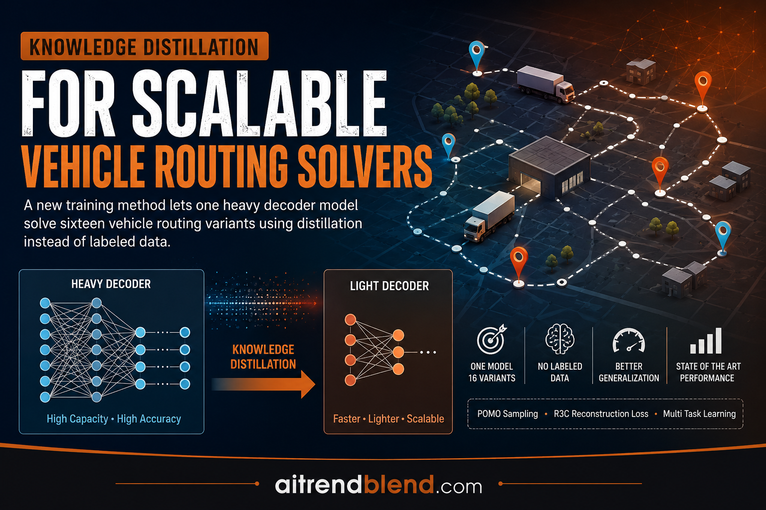
- MTL-KD trains a single heavy decoder model to solve sixteen vehicle routing problem variants using knowledge distillation from six specialist teacher models instead of labeled routes.
- Heavy decoder architectures generalize far better to large problems than the light decoder designs most multi task routing models use, but they were previously too expensive to train with reinforcement learning across many tasks at once.
- The student model is supervised by matching its output probabilities to each teacher’s output probabilities, which sidesteps the need for optimal solution labels entirely.
- A new inference trick called Random Reordering Reconstruction shuffles the order of route segments during refinement, which improves solution quality further without retraining.
- On problems with a thousand nodes, MTL-KD cuts the performance gap to the best heuristic solver roughly in half compared to the strongest prior multi task neural baselines.
The problem nobody wanted to admit was a training problem
Vehicle routing sounds like a solved problem until you actually try to solve it at scale. A logistics company does not have one routing problem. It has a family of them. Some trucks return to a central warehouse and some do not. Some customers demand a delivery within a specific two hour window. Some routes carry a mix of outgoing shipments and returned goods that has to be sequenced carefully. Combine four of these constraints on top of the base capacitated vehicle routing problem and you get sixteen distinct variants, each one NP hard on its own.
For years the dominant approach in neural combinatorial optimization has been what researchers call a heavy encoder with a light decoder. The encoder does most of the thinking up front, producing a rich embedding for every node, and a thin decoder quickly reads those embeddings off one node at a time to build a route. POMO, introduced by Kwon and colleagues in 2020, is the model most of this later work builds on. It works beautifully on problems around one hundred nodes. The trouble starts when you scale up. A light decoder simply does not have enough capacity to make sense of thousands of dense, high resolution node embeddings, and its quality falls apart on large instances.
The opposite design, a light encoder paired with a heavy decoder, fixes that weakness. Luo and colleagues showed in 2023 that a decoder which keeps re evaluating the relationship between remaining nodes and the current position at every single step generalizes to much larger problems than a light decoder ever could. The catch is cost. A heavy decoder recomputes attention over every unvisited node at every decoding step, which makes training it with reinforcement learning across an entire construction trajectory extremely expensive. Supervised learning would sidestep that cost, but there are no ground truth optimal routes for most of these problem variants, and generating them at scale is itself a hard combinatorial search problem. One prior attempt, called SIT, tried to bootstrap its own labels through local reconstruction, but early in training those self generated labels are low quality, which drags out the whole process.
So the field was stuck between two bad options. Train a light decoder cheaply and watch it fail on large problems, or train a heavy decoder well and pay a cost nobody could afford across sixteen problem variants at once. MTL KD is the paper’s answer to that standoff, and the fix is almost embarrassingly simple once you see it. Do not train the heavy decoder from scratch on all sixteen problems. Train six cheap specialist models first, one per base task, using ordinary reinforcement learning the way POMO already does. Then have the expensive heavy decoder model learn by copying those specialists rather than by exploring the search space itself.
How the distillation pipeline actually works
Six teachers, one classroom
The setup starts with six seen tasks, CVRP, OVRP, VRPB, VRPL, VRPTW, and OVRPTW, each covering one of the four extra constraints researchers care about, open routes, backhauls, duration limits, and time windows, plus the plain base problem and one combination case. For each of these six tasks the team trains an independent POMO style teacher using the standard policy gradient method from Williams, with a shared baseline computed across multiple starting trajectories per instance. Every teacher gets six encoder layers, one light decoder layer, and trains for four thousand epochs on randomly generated instances of one hundred nodes.
These teacher models are unremarkable on their own. They are exactly what you would build if you wanted a fast, cheap POMO baseline for a single task. Their real value only shows up once the student starts learning from them.
The student learns by watching, not by exploring
The student model has a completely different shape. Instead of six encoder layers and one decoder layer, it flips the ratio, using one encoder layer and six decoder layers, which is the heavy decoder pattern that gives strong scale generalization. During training, every batch contains instances from all six seen tasks at once. At each decoding step the student produces a probability distribution over which node to visit next, and so does the matching teacher for that specific task, evaluated on the exact same partial solution state.
The student is never told which node is correct. It is only told how confident each teacher was about each option, and it is trained to match that confidence profile as closely as possible using a Kullback Leibler divergence loss summed across all six teachers.
Here each of the M teacher policies supervises the student policy on its own task, so a VRPTW instance is judged against the VRPTW teacher and a backhaul instance is judged against the backhaul teacher. This is the whole trick. There is no reward signal, no exploration, and no labeled tour anywhere in the loop. The student simply gets pulled toward whatever distribution the relevant specialist already believes in.
What the heavy decoder is actually doing under the hood
The architecture itself follows the pattern established by earlier heavy decoder work, with some VRP specific plumbing bolted on. The encoder is deliberately thin, a single Transformer layer mapping raw node features, coordinates, demand, service time, and time window bounds, into an initial embedding.
The decoder is where the real computation happens. At every step it pulls together the embeddings of unvisited nodes, the last visited node, and the depot node, each combined with dynamic features covering remaining vehicle capacity, current time, remaining route duration, and whether the route is allowed to stay open. These get passed through an L layer Transformer network, with a padding mask handling the fact that different instances in a batch have different numbers of unvisited nodes remaining.
The compatibility score c comes from single head attention between each unvisited node’s final embedding and a context vector built from the last visited node and the depot. Two masks get added before the softmax. One handles padding so instances of different lengths can share a batch, and one enforces feasibility, blocking moves that would violate capacity, a time window, or a duration limit. The paper also notes a small but meaningful architectural choice, dropping layer normalization from every attention layer, a detail carried over from the original heavy decoder work by Luo and colleagues, which apparently helps stability at this depth.
Random Reordering Reconstruction, a cheap trick with a real payoff
Training the model well is only half the story. At inference time, the paper also proposes an improvement strategy called Random Reordering Reconstruction, or R3C, which builds on an older idea called Random Reconstruction from the original heavy decoder paper.
Random Reconstruction works by taking a full solution, decomposing it into its individual subtours, randomly sampling a contiguous segment, and letting the model re optimize just that segment while holding the rest fixed. If the re optimized segment improves the total distance, it replaces the original. This is iterative local search dressed up in a neural policy, and it works well, but it has a real limitation. Randomly reversing a subtour can produce an infeasible route for constrained problems like VRPTW, where the order customers are visited in actually matters because of their time windows.
R3C keeps the same core loop but adds one change with an outsized effect. Before sampling a segment to re optimize, it first randomizes the external order of the subtours themselves, not the customers within them. So instead of always sampling from the same fixed sequence of subtours, the model gets to see many different combinations of which subtour comes before which. That single change meaningfully increases the diversity of partial solutions the model gets to explore during refinement, without breaking feasibility for problems where reversing a subtour outright is not safe. Feasible subtour reversals are still applied where they are legal, so the method keeps the best of both approaches rather than choosing one over the other.
What the numbers actually show
The experiments run across sixteen VRP variants at four problem sizes, one hundred, two hundred, five hundred, and one thousand nodes, benchmarked against HGS PyVRP as the strong traditional heuristic baseline, Google’s OR Tools, and four neural multi task competitors, MT POMO, MVMoE, RouteFinder, and CaDA. The headline pattern across nearly every table is the same. The gap between MTL KD and the traditional solver grows very slowly as problem size increases, while the gap for every other neural baseline grows fast.
| Method | CVRP gap at 100 nodes | CVRP gap at 500 nodes | CVRP gap at 1000 nodes |
|---|---|---|---|
| MT POMO with augmentation | 1.69 percent | 9.54 percent | 14.28 percent |
| MVMoE with augmentation | 1.50 percent | 18.59 percent | 47.57 percent |
| RF MVMoE with augmentation | 2.01 percent | 8.52 percent | 12.80 percent |
| MTL KD with R3C, 200 iterations | 1.48 percent | 2.51 percent | 2.10 percent |
That last row is the interesting one. On the smallest instances MTL KD is roughly tied with the best competitors. As the problem grows the other models degrade steadily, while MTL KD barely moves, ending up almost six times closer to the heuristic baseline than MVMoE at one thousand nodes. The same pattern repeats across the ten unseen task variants the model never saw during training, which is arguably the more important test since it is the closest analog to what happens when a company adds a new constraint their planning software was not built for.
The paper also runs a direct comparison that isolates the value of distillation itself. They train the same heavy decoder architecture two ways, once with knowledge distillation and once with plain reinforcement learning, and because RL training on the heavy decoder is so expensive they could only push the RL version to instances of size twenty. At problem size one hundred, the RL trained version had an average gap of 21.8 percent on training tasks, while the distilled version had a gap of 5.5 percent. On unseen tasks at one thousand nodes the RL version’s gap ballooned to 62.2 percent, compared to 13.3 percent for the distilled version. Distillation was not just a cheaper way to reach the same destination. It reached a meaningfully better destination.
Real world testing tells a similar story. On CVRPLIB’s Set-X benchmark, a widely used collection of realistic instances rather than randomly generated ones, MTL KD achieved an average gap of 4.025 percent, well ahead of MVMoE’s 4E variant at 6.884 percent and its larger 4E-L variant at 5.160 percent. On the larger scale Set-X instances the gap stretched further, with MTL KD at 6.655 percent against 12.303 percent for the next closest competitor, RouteFinder’s Transformer variant. On the Solomon VRPTW benchmark, a decades old but still widely referenced test set with strict time constraints, MTL KD posted an average gap of 15.786 percent against 18.490 percent for the best MVMoE variant, a meaningful improvement on problems that are notoriously punishing for models that were only trained on uniformly random synthetic data.
What this means beyond the leaderboard
Step back from the tables and the underlying idea generalizes well past vehicle routing. Whenever you have several cheap, well trained specialist policies and want to merge their capability into one larger, more capable model, distillation through output matching sidesteps the need for labeled examples entirely. That matters most in exactly the settings where labels are hardest to get, which in combinatorial optimization is almost everywhere, since finding a provably optimal solution to an NP hard problem at scale is itself the whole difficulty.
There is also a practical operations lesson buried in here for anyone maintaining a routing system with multiple constraint types in production. The traditional path is either maintain six separate specialist solvers or accept the quality hit that comes with a single generalist light decoder model. MTL KD points at a third option, train the specialists you already know how to train cheaply, then spend your heavier compute budget once, on a distillation pass, rather than repeatedly on reinforcement learning across every task combination you might eventually need.
The R3C inference strategy is worth separate attention from practitioners who are not training their own models at all. It is a post hoc refinement trick that works on top of an already trained heavy decoder, and the core idea, randomizing structural order before sampling a subproblem to refine, is portable to other constructive combinatorial solvers well beyond VRP variants specifically.
Honest limitations
The heavy decoder architecture that makes MTL KD generalize so well to large problems is also its biggest practical cost. Recomputing attention over all unvisited nodes at every decoding step is expensive at inference time, and the paper is upfront about this in its own conclusion, flagging high computational complexity as the main direction for future work. A company deploying this in a real time dispatch system would need to weigh that latency against the accuracy gains, especially for very large fleets where routing decisions need to happen quickly.
The training setup also depends entirely on the quality of the six teacher models. If a teacher has a systematic blind spot on its own task, that blind spot has no mechanism to be corrected during distillation, since the student is explicitly trained to match the teacher’s distribution rather than to independently discover better solutions. The scale generalization result is encouraging precisely because it was not guaranteed, but it is one experiment on one architecture, and it would be worth seeing whether the same generalization gap between teacher and student holds on problem families with very different structure than vehicle routing.
Finally, all sixteen variants studied here share the same underlying capacitated vehicle routing skeleton with different constraints layered on top. That is a reasonable and practically important test bed, but it is still a family of closely related problems. Whether knowledge distillation from specialist teachers generalizes this cleanly across genuinely unrelated combinatorial optimization problem classes, say routing alongside scheduling or bin packing in the same student model, remains an open question the current paper does not attempt to answer.
Complete PyTorch implementation
The code below is a compact, runnable reimplementation of the core ideas in the paper. It includes a simplified heavy decoder student model, a lightweight teacher stand in, the knowledge distillation loss from the paper, a training loop, an evaluation function computing tour length, and a smoke test that runs the whole pipeline on randomly generated dummy CVRP instances. It is meant to demonstrate the mechanics clearly rather than to match the paper’s exact hyperparameters or performance.
import torch
import torch.nn as nn
import torch.nn.functional as F
import math

# ---------------------------------------------------------------
# Shared building block, a lightweight Transformer style layer
# used inside both the teacher and the student decoder stacks.
# ---------------------------------------------------------------
class TransformerBlock(nn.Module):
    def __init__(self, dim, heads=8, ff_dim=512):
        super().__init__()
        self.attn = nn.MultiheadAttention(dim, heads, batch_first=True)
        self.ff = nn.Sequential(
            nn.Linear(dim, ff_dim), nn.ReLU(), nn.Linear(ff_dim, dim)
        )

    def forward(self, x, key_padding_mask=None):
        # Layer normalization is intentionally omitted, following the
        # paper's note that removing it improved stability for the
        # heavy decoder stack.
        attn_out, _ = self.attn(x, x, x, key_padding_mask=key_padding_mask)
        x = x + attn_out
        x = x + self.ff(x)
        return x


# ---------------------------------------------------------------
# Teacher, a small POMO style model with a heavy encoder and a
# light single layer decoder. One of these would be trained per
# seen task in the real pipeline.
# ---------------------------------------------------------------
class TeacherModel(nn.Module):
    def __init__(self, node_dim=3, embed_dim=128, encoder_layers=6):
        super().__init__()
        self.input_proj = nn.Linear(node_dim, embed_dim)
        self.encoder = nn.ModuleList(
            [TransformerBlock(embed_dim) for _ in range(encoder_layers)]
        )
        self.decoder_head = nn.Linear(embed_dim, embed_dim)

    encode = None  # placeholder attribute, real method defined below

    def encode(self, nodes):
        h = self.input_proj(nodes)
        for layer in self.encoder:
            h = layer(h)
        return h

    def forward(self, nodes, last_idx, unvisited_mask):
        # nodes, shape (batch, n, node_dim)
        # last_idx, shape (batch,), index of last visited node
        # unvisited_mask, shape (batch, n), True where a node is still open
        h = self.encode(nodes)
        batch_size = nodes.size(0)
        last_embed = h[torch.arange(batch_size), last_idx]
        query = self.decoder_head(last_embed).unsqueeze(1)
        logits = torch.bmm(query, h.transpose(1, 2)).squeeze(1)
        logits = logits.masked_fill(~unvisited_mask, float('-inf'))
        return F.log_softmax(logits, dim=-1)


# ---------------------------------------------------------------
# Student, the multi task heavy decoder. One shared thin encoder,
# several decoder layers that re attend over unvisited nodes at
# every step, matching the paper's inverted encoder decoder ratio.
# ---------------------------------------------------------------
class HeavyDecoderStudent(nn.Module):
    def __init__(self, node_dim=3, embed_dim=128, decoder_layers=6):
        super().__init__()
        self.input_proj = nn.Linear(node_dim, embed_dim)
        self.encoder = TransformerBlock(embed_dim)
        self.decoder = nn.ModuleList(
            [TransformerBlock(embed_dim) for _ in range(decoder_layers)]
        )
        self.context_proj = nn.Linear(embed_dim * 2, embed_dim)
        self.score_proj = nn.Linear(embed_dim, embed_dim)

    def forward(self, nodes, last_idx, depot_idx, unvisited_mask):
        h0 = self.input_proj(nodes)
        h = self.encoder(h0)
        for layer in self.decoder:
            h = layer(h, key_padding_mask=~unvisited_mask)
        batch_size = nodes.size(0)
        last_embed = h[torch.arange(batch_size), last_idx]
        depot_embed = h[torch.arange(batch_size), depot_idx]
        context = self.context_proj(torch.cat([last_embed, depot_embed], dim=-1))
        query = self.score_proj(context).unsqueeze(1)
        logits = torch.bmm(query, h.transpose(1, 2)).squeeze(1)
        logits = logits.masked_fill(~unvisited_mask, float('-inf'))
        return F.log_softmax(logits, dim=-1)


# ---------------------------------------------------------------
# The distillation loss from Section 3.3 of the paper, KL divergence
# between each teacher and the student, summed across tasks.
# ---------------------------------------------------------------
def distillation_loss(student_log_probs, teacher_log_probs):
    teacher_probs = teacher_log_probs.exp()
    kl = F.kl_div(student_log_probs, teacher_probs, reduction='batchmean')
    return kl


# ---------------------------------------------------------------
# Tour length evaluation, used to check solution quality once a
# full route has been constructed.
# ---------------------------------------------------------------
def tour_length(coords, tour):
    # coords, shape (n, 2) . tour, list of node indices ending at depot
    total = 0.0
    for a, b in zip(tour[:-1], tour[1:]):
        total += math.dist(coords[a].tolist(), coords[b].tolist())
    return total


# ---------------------------------------------------------------
# Training loop, one epoch of distillation on random CVRP style
# instances. A real run would loop across all six seen tasks and
# their matching teachers within every batch.
# ---------------------------------------------------------------
def train_one_epoch(student, teacher, optimizer, batch_size=32, n_nodes=20, steps=10):
    student.train()
    teacher.eval()
    running_loss = 0.0
    for _ in range(steps):
        coords = torch.rand(batch_size, n_nodes, 2)
        demand = torch.rand(batch_size, n_nodes, 1)
        nodes = torch.cat([coords, demand], dim=-1)

        last_idx = torch.zeros(batch_size, dtype=torch.long)
        depot_idx = torch.zeros(batch_size, dtype=torch.long)
        unvisited_mask = torch.ones(batch_size, n_nodes, dtype=torch.bool)
        unvisited_mask[:, 0] = False

        with torch.no_grad():
            teacher_log_probs = teacher(nodes, last_idx, unvisited_mask)

        student_log_probs = student(nodes, last_idx, depot_idx, unvisited_mask)

        loss = distillation_loss(student_log_probs, teacher_log_probs)
        optimizer.zero_grad()
        loss.backward()
        optimizer.step()
        running_loss += loss.item()

    return running_loss / steps


# ---------------------------------------------------------------
# Evaluation, greedily construct one full route with the student
# model and report its length.
# ---------------------------------------------------------------
def evaluate_greedy(student, n_nodes=20):
    student.eval()
    coords = torch.rand(1, n_nodes, 2)
    demand = torch.rand(1, n_nodes, 1)
    nodes = torch.cat([coords, demand], dim=-1)

    depot_idx = torch.zeros(1, dtype=torch.long)
    last_idx = depot_idx.clone()
    unvisited_mask = torch.ones(1, n_nodes, dtype=torch.bool)
    unvisited_mask[0, 0] = False
    tour = [0]

    with torch.no_grad():
        while unvisited_mask.any():
            log_probs = student(nodes, last_idx, depot_idx, unvisited_mask)
            next_idx = log_probs.argmax(dim=-1)
            tour.append(next_idx.item())
            unvisited_mask[0, next_idx] = False
            last_idx = next_idx
    tour.append(0)
    return tour_length(coords[0], tour), tour


# ---------------------------------------------------------------
# Smoke test, runs the full pipeline end to end on dummy data to
# confirm every piece connects correctly.
# ---------------------------------------------------------------
if __name__ == '__main__':
    torch.manual_seed(0)
    teacher = TeacherModel()
    student = HeavyDecoderStudent()
    optimizer = torch.optim.Adam(student.parameters(), lr=1e-4)

    avg_loss = train_one_epoch(student, teacher, optimizer, batch_size=8, n_nodes=15, steps=5)
    print('average distillation loss over smoke test epoch', avg_loss)

    length, tour = evaluate_greedy(student, n_nodes=15)
    print('greedy tour length on a random instance', length)
    print('tour', tour)

    assert len(tour) == 16, 'expected every node visited plus a return to the depot'
    assert length > 0, 'tour length should be a positive number'
    print('smoke test passed')
Conclusion
The core achievement here is narrower and more useful than it might first sound. MTL KD does not invent a new way to solve vehicle routing problems. It solves a training problem that was quietly blocking a design everyone already suspected was better. Heavy decoder architectures were known to generalize well to large scale instances well before this paper. What was missing was an affordable way to train one across many task variants at once, and knowledge distillation from cheap specialist teachers turns out to be exactly that missing piece.
The conceptual shift worth remembering is that distillation here is not being used for its usual purpose of compression, squeezing a big model into a small one for deployment. It is being used as a training strategy in its own right, a way of converting expensive multi task reinforcement learning into a cheaper supervised style problem by letting a teacher’s own output distribution stand in for a label that does not exist. That reframing is portable well beyond routing. Anywhere a field has strong single task specialists but no ground truth labels for the combined multi task version of the problem, this same pattern of train specialists first, then distill into a unified model, is worth trying.
Transferability is the part most worth watching going forward. The paper stays inside a tightly related family of sixteen CVRP variants, which is a fair scope for a first paper but leaves open how far the approach travels. Scheduling problems, bin packing, network design, and other combinatorial domains with a similar mismatch between architecture quality and training cost seem like natural next candidates, and the R3C inference trick in particular reads as generally applicable to any constructive solver that builds a solution as an ordered sequence of decisions.
The honest limitations are real and the authors do not hide from them. A heavy decoder is expensive at inference time no matter how it was trained, the student’s ceiling is bounded by whatever blind spots its teachers carry, and the generalization result, while striking, rests on one architecture tested on one problem family. None of that undercuts what was actually demonstrated, but it does mean the interesting open questions are about how far this pattern extends rather than whether it works at all within its tested scope.
What sticks with you after reading this paper is not the leaderboard numbers, strong as they are, but the framing choice underneath them. Instead of asking how to make a heavy decoder cheaper to train with reinforcement learning, the authors asked what a heavy decoder actually needs supervision from, and realized the answer was sitting right there in six models they already knew how to train.
Go deeper
Read the full paper for the complete experimental tables and the appendix ablations on segment length and inference strategy.
Frequently asked questions
What problem does MTL KD actually solve
It solves the problem of training a single heavy decoder neural network to handle many different vehicle routing problem variants at once, without needing labeled optimal routes, by having the model learn to imitate several smaller specialist models instead of exploring the search space with reinforcement learning directly.
Why not just train the heavy decoder with reinforcement learning like the teachers
The paper’s own ablation shows this is where the approach breaks down. Because a heavy decoder recomputes attention over all unvisited nodes at every step, reinforcement learning across an entire trajectory becomes too expensive to run at a useful problem scale, and the resulting model performs far worse than the distilled version even when the RL version is given a smaller training scale to work with.
Does the student model only work on the six tasks it was trained on
No. The paper tests it on ten additional unseen VRP variants that combine constraints in new ways, and MTL KD outperforms the other multi task neural baselines on most of them, particularly at larger problem sizes, suggesting the model learned something more general than the six specific tasks it saw during training.
What is Random Reordering Reconstruction in plain terms
It is an inference time refinement trick. After a solution is built, the model breaks it into subtours, shuffles the order those subtours appear in, then samples a segment to re optimize. Shuffling first gives the model a wider variety of partial solutions to refine from, which improves final solution quality without any additional training.
How much better is MTL KD than prior multi task routing models
On the seen training tasks at one thousand nodes it roughly halves the performance gap to the strongest heuristic baseline compared to the best prior multi task neural competitor in the paper’s tables, and it shows a similar advantage on real world benchmarks like CVRPLIB Set-X and the Solomon VRPTW dataset.
Is this approach limited to vehicle routing specifically
The specific architecture and constraints are tailored to VRP variants, but the underlying training idea, distilling several cheap single task specialists into one expensive multi task model instead of training that model directly with reinforcement learning, is a general pattern that could plausibly extend to other combinatorial optimization problems with the same training cost mismatch.
This analysis is based on the published paper and an independent evaluation of its claims.
Pingback: Unlock 57.2% Reasoning Accuracy: KDRL Revolutionary Fusion Crushes LLM Training Limits - aitrendblend.com