
Key points
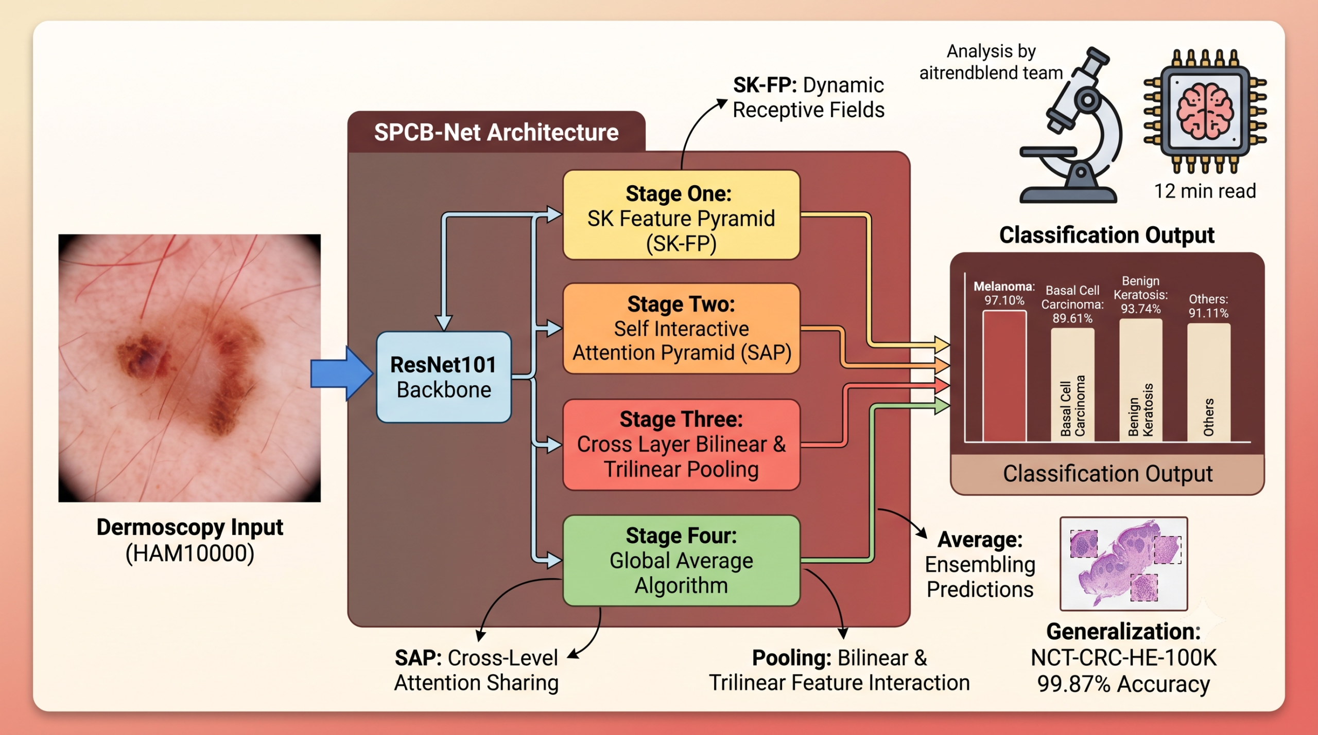
- SPCB-Net combines a feature pyramid, a self interactive attention pyramid, and a cross layer bilinear and trilinear pooling operation to classify skin lesion images.
- On the HAM10000 dermoscopy dataset the ResNet101 version reached 97.10 percent accuracy, about 0.4 percentage points above the comparison models the authors cite.
- The same architecture was tested on a completely different task, sorting colorectal tissue patches in the NCT-CRC-HE-100K dataset, and reached 99.87 percent accuracy.
- Ablation experiments show the attention pyramid and the pooling operation each contribute measurable gains on their own, and the biggest jump comes from a five way averaging step the authors call the global average algorithm.
- The paper is a peer reviewed engineering study on public benchmark data, not a clinical trial, and none of its numbers should be read as a diagnostic guarantee for any individual patient.
Why low level and high level features fight each other
Every convolutional network builds a stack of feature maps as an image moves through its layers. The early layers see fine texture, edges, small color patches, the kind of detail a dermatologist notices when zooming in on a lesion border. The later layers see something closer to a compressed summary, shapes and rough regions rather than pixels, because each layer has a wider view of the original image and a smaller resolution to work with. Xin Qian and coauthors point out a specific failure mode in skin images. In many pairs of dermoscopy photos, the low level texture of two different disease categories looks nearly the same, hair, skin tone, lighting artifacts and all, while the high level shape signature of two photos from the very same category can look quite different from patient to patient. Figure 2 in the paper shows this directly, with rows of lesions from the same class that share almost nothing in outline or color once you get past the surface texture.
That mismatch is the core obstacle the authors are responding to. A plain classifier trained end to end tends to lean on whichever level of feature happens to separate the training set best, and if the true signal is split across both levels the network has no built in mechanism for combining them. SPCB-Net is an attempt to give the network that mechanism explicitly, through three linked pieces, a feature pyramid tuned by a selective kernel module, an attention structure that lets different depth levels talk to each other, and a pooling step that multiplies features from different layers together instead of just concatenating them.
The five stage pipeline
Look at Figure 3 in the paper and you can trace the whole system in one image. A backbone, either VGG19 or ResNet101 in the experiments, produces four feature maps B1 through B4 at different depths and resolutions. From there the pipeline runs through four stages before it ever reaches a classifier.
Stage one, the SK feature pyramid
The first new piece is what the authors call SK-FP, a mashup of a standard feature pyramid network and Selective Kernel Networks, or SKNet. A regular feature pyramid takes deep, low resolution maps and merges them into shallow, high resolution ones through upsampling and addition, which is the same recipe object detectors have used since 2017. The complaint the authors raise is that a normal pyramid applies the same convolution kernel size at every scale, and a single kernel size is not equally good at capturing a five pixel texture pattern and a two hundred pixel lesion outline. SKNet solves that by learning, per channel, how much weight to give a small receptive field versus a large one, effectively letting the network choose its own kernel size on the fly. The paper’s equation 1 describes each input map being passed through this selective kernel operation, and equation 3 describes how the resulting maps are fused top down with progressive upsampling, producing four pyramid outputs labeled F1 through F4 that carry both fine texture and broad shape information at every scale.
Stage two, the self interactive attention pyramid
Here is where it gets interesting. Attention modules like Squeeze and Excitation from Hu and colleagues in 2018, or the Convolutional Block Attention Module from Woo and colleagues, already know how to reweight a single feature map along its channel axis, its spatial axis, or both. What none of them do by default is let attention computed at one depth influence attention computed at another depth. SPCB-Net’s self interactive attention pyramid, SAP for short, adds exactly that connection. At each of the four pyramid levels the network computes a spatial attention mask, following the CBAM recipe but with a 3 by 3 convolution kernel swapped in for the original 7 by 7 kernel to cut compute, and a channel attention mask built from average pooling followed by two convolution layers in the SE and ECA tradition. Then, and this is the part that makes it a pyramid rather than four independent attention blocks, the authors add a skip connection that blends the attention mask from one level with the mask one level below it, averaging the two according to equations 7 and 8 in the paper. The ablation study found the best configuration links only the first two levels, D1 and D2, rather than chaining all four together, which the authors attribute to diminishing returns and possible noise once too many levels get mixed.
Once the spatial and channel masks are computed, they get added together and multiplied element wise back onto the original feature map, so a region that scores high on both spatial importance and channel importance gets amplified while a region that scores low on both gets suppressed. That is a fairly standard attention gating step, the novelty sits entirely in the cross level averaging that happens before this final multiplication.
Stage three, cross layer bilinear and trilinear pooling
This is the piece the paper’s title leads with, and it deserves the most explanation because it is genuinely the least intuitive part of the architecture. Bilinear pooling, going back to work by Lin, RoyChowdhury and Maji in 2015, takes two feature maps and multiplies them together element by element, the Hadamard product, then averages the result. The idea is to capture second order interaction, which pixel activations tend to co occur, rather than just first order presence or absence of a feature. Trilinear pooling extends the same trick to three feature maps at once, capturing third order interaction, and Wang and colleagues showed in prior fine grained classification work that trilinear pooling tends to outperform bilinear pooling because it captures richer correlation, at the cost of needing more computation and more parameters.
SPCB-Net’s contribution here is a compromise rather than a pure choice of one over the other. Two of the four output pooling results, D1 and D2, are computed with plain bilinear pooling between two channel attention maps. The other two, D3 and D4, are computed with trilinear pooling between three channel attention maps. The formulas are direct.
The ablation table the authors report, labeled 12 BT 34 in their notation meaning bilinear pooling at positions one and two and trilinear pooling at positions three and four, beat every other combination they tried, including pure bilinear pooling everywhere and pure trilinear pooling everywhere. The reasoning offered is that applying full trilinear pooling across all four attention maps adds computational cost without a matching accuracy gain, so mixing the two operations captures most of the benefit of trilinear interaction while keeping part of the network cheap. It is a pragmatic choice more than an elegant one, and the paper is honest that the accuracy difference this specific step contributes on its own is modest next to what the attention pyramid contributes, something the ablation numbers below make clear.
Stage four, the global average algorithm
The last piece is almost embarrassingly simple compared to everything before it, and the ablation results suggest it might matter the most. Rather than sending one final feature vector to one classifier, SPCB-Net builds five separate lightweight classifiers, each a global pooling layer followed by two fully connected layers. One classifier reads directly from the backbone output D0, and one reads from each of the four pooled interaction outputs D1 through D4. All five produce a prediction, the five predictions get summed, and the sum is divided by five to produce the final averaged prediction. This is essentially a built in ensemble, five weak classifiers voting instead of one strong classifier deciding alone, and the cross entropy loss used during training is applied to constrain all five outputs jointly rather than only the final average.
Why an internal ensemble helps
Averaging five classifiers that each see a slightly different slice of the network, raw backbone features versus various pooled interaction features, tends to smooth out the mistakes any single classifier makes on ambiguous inputs. It is the same intuition behind bagging in classical machine learning, applied inside a single forward pass instead of across separately trained models.
The datasets and how the images were prepared
The primary target dataset is HAM10000, short for Human Against Machine with 10000 training images, a widely used dermoscopy collection assembled by Tschandl, Rosendahl and Kittler and published in Scientific Data in 2018. It contains 10015 images at 450 by 600 pixels across seven diagnostic categories, melanoma, melanocytic nevi, basal cell carcinoma, actinic keratosis and intraepithelial carcinoma, benign keratosis, dermatofibroma, and vascular lesions. More than half the ground truth labels in the dataset come from histopathology confirmation, with the rest confirmed through follow up exams, expert consensus, or confocal microscopy. The authors split it 80 percent training, 10 percent validation, and 10 percent test, giving 8017 training images, 999 validation images, and 999 test images.
Because dermoscopy images frequently include body hair that obscures the lesion border, the preprocessing pipeline applies two hair removal techniques before training, a black hat morphological operation and a closed operation that expands the image before eroding it back down. Figures 8 and 9 in the paper show the visible effect, stripping out hair strands while leaving the lesion itself intact. Standard augmentation follows, random horizontal flips at a 0.5 probability along with randomized brightness, contrast, saturation, and hue jitter at a 0.4 probability, aimed at reducing overfitting on a dataset that, at ten thousand images, is small by deep learning standards.
To test whether the architecture generalizes beyond dermatology, the same network was evaluated on NCT-CRC-HE-100K, a histopathology dataset of 100000 image patches drawn from 86 hematoxylin and eosin stained colorectal cancer tissue slides sourced from the National Center for Tumor Diseases biobank and the University Medical Center Mannheim archive. This dataset covers nine tissue categories rather than seven disease categories, normal colonic mucosa, tumor associated stroma, colorectal adenocarcinoma epithelium, adipose tissue, background, tissue fragments, lymphocytes, mucus, and smooth muscle. Because this dataset is already large and reasonably balanced, no augmentation was applied to it.
What the numbers actually show
Table 1 in the paper compares SPCB-Net against five common backbone architectures trained on the same HAM10000 split, VGG19, ResNet101, ShuffleNet_v2, GoogLeNet, and DenseNet121, none of which include any of SPCB-Net’s added modules. The plain backbones range from ShuffleNet_v2 at 88.59 percent accuracy up to ResNet101 at 95.40 percent. Every version of SPCB-Net beats every plain backbone, and the ResNet101 based version reaches 97.10 percent accuracy with 93.66 percent precision, 93.34 percent recall, 99.40 percent specificity, and an F1 score of 92.25 percent, the best across every metric the authors report.
| Model | Accuracy | Precision | Recall | F1 |
|---|---|---|---|---|
| VGG19 backbone alone | 86.99% | 75.26% | 73.37% | 73.91% |
| ResNet101 backbone alone | 95.40% | 89.61% | 91.11% | 89.89% |
| DenseNet121 backbone alone | 93.74% | 87.37% | 83.64% | 85.36% |
| SPCB-Net with VGG19 | 96.80% | 93.06% | 92.49% | 92.76% |
| SPCB-Net with ResNet101 | 97.10% | 93.66% | 93.34% | 92.25% |
The ablation results in Table 5 are arguably more informative than the headline number, because they isolate what each piece is actually doing. Starting from a plain ResNet101 at 95.40 percent accuracy, adding just the SK feature pyramid brings it to 96.45 percent. Adding the attention pyramid on top of that reaches 96.75 percent. Swapping in the pooling operation instead of the attention pyramid, while keeping the pyramid, reaches 96.55 percent, showing the two additions contribute roughly comparable but not identical gains on their own. Only the full combination, all three pieces together, reaches the reported 97.10 percent. None of the individual pieces is doing all the work, which is a reasonably honest way for the ablation to shake out and suggests the modules are at least partially complementary rather than redundant.
Against outside comparison models the authors cite, DenseNet II at 96.27 percent accuracy, a dual position encoding bottleneck transformer network called DPE BoTNeT at 95.80 percent, FixCaps at 96.49 percent, and a cubic support vector machine pipeline at 96.70 percent, SPCB-Net with ResNet101 comes out ahead by roughly 0.4 percentage points, which is the improvement figure the abstract highlights. It is worth being honest about what that margin means. Four tenths of a percentage point on a 999 image test set is a real but modest gap, and it sits within a range where dataset split choices, augmentation randomness, or minor training differences between labs could plausibly move results by a similar amount. The paper does not report confidence intervals or repeated run variance for these comparisons, so the 0.4 percent figure should be read as a point estimate on one test split rather than a statistically guaranteed advantage.
On the colorectal tissue dataset the numbers look stronger in absolute terms, 99.87 percent accuracy for the ResNet101 version and 99.83 percent for the VGG19 version, both edging out comparison methods like an ensemble deep neural network at 99.13 percent, a clustering based method called DARC at 99.76 percent, and an interactive multi channel attention approach called IL MCAM at 99.78 percent. Ceiling effects are worth flagging here too, once accuracy sits above 99.7 percent across several competing methods, the remaining differences are small in absolute image count even if they look meaningful as percentages, since NCT-CRC-HE-100K’s test portion contains 9995 images and a 0.1 percentage point gap corresponds to roughly ten images either way.
Clinical translation gap
None of this closes the distance between a benchmark result and a tool a dermatology clinic could actually deploy. HAM10000 is a curated, cleaned, and expert labeled research dataset drawn from a handful of centers, and dermoscopy image quality, lighting, and camera hardware vary considerably across real world clinical settings in ways the training data may not fully represent. The paper does not report performance broken down by skin tone, patient age, lesion size, or image source device, all of which are known sources of performance disparity in dermatology AI systems more broadly. It also does not report external validation on a separate dataset collected at a different institution, which is generally considered a stronger test of real world generalization than a held out split from the same source dataset. A model reaching 97 percent accuracy on a research benchmark is a meaningful engineering result and a long way from a validated clinical decision support product, and the authors themselves frame the work as a step toward computer aided diagnosis rather than a finished diagnostic tool.
Key takeaway
The 0.4 percentage point improvement over prior models, repeated on two very different datasets, is the strongest evidence in the paper that the architecture generalizes as a general purpose feature interaction module rather than something tuned specifically to skin images. That said, both improvements are measured against each dataset’s own held out split, not against an independent external cohort.
Honest limitations
The authors flag one limitation explicitly in their conclusion, that the paper does not analyze the computational complexity of SPCB-Net or test its effectiveness on tasks outside the two datasets used, and they list a theoretical complexity analysis as future work. A few additional constraints are worth naming even though the paper does not dwell on them. The HAM10000 test set used for the headline 97.10 percent figure contains only 999 images spread across seven classes with a heavily skewed distribution, melanocytic nevi alone make up about 67 percent of the dataset according to the paper’s own Figure 6, while dermatofibroma and vascular lesions each make up only a few percent. Rare class performance in a skewed dataset like this is exactly where accuracy as a single headline number can be misleading, since a model that does very well on the majority class can still post a high overall accuracy while making meaningful errors on the minority classes that matter most clinically. The confusion matrices in Figure 10 do show this pattern to some extent, with dermatofibroma and vascular lesion classes showing more confusion than melanocytic nevi across most of the compared models. The paper also trains and tests within a single dataset source for each benchmark, so cross institution or cross device generalization remains untested, and it uses cross entropy loss without any explicit class weighting to counter the label imbalance described above.
Where this fits and what comes next
Zoom out and SPCB-Net reads less like a dermatology specific invention and more like a general recipe for combining multiscale feature interaction with attention, applied to two medical imaging tasks as a proof of concept. The fact that the same architecture, retrained but not redesigned, performed well on colorectal histopathology patches as well as dermoscopy images is the paper’s best argument for that broader framing. If the underlying idea generalizes, the natural next test would be applying the same pyramid and pooling combination to other imaging domains where small class differences and large within class variation both show up, retinal imaging for diabetic retinopathy grading or chest imaging for early stage findings both come to mind as domains with a similar intra class versus inter class tension. The authors do not test either of those directly, so that remains a reasonable hypothesis rather than a demonstrated result. What is demonstrated is a fairly careful set of ablation experiments that isolate what each architectural piece contributes, which is more useful to other researchers building on this work than the headline accuracy figure alone.
Conclusion
SPCB-Net’s core achievement is showing that three separately reasonable ideas, a selective kernel feature pyramid, a cross level attention structure, and a mixed bilinear and trilinear pooling operation, combine into a measurable improvement over strong existing backbones on both a dermatology benchmark and an unrelated histopathology benchmark. The conceptual shift worth noticing is the treatment of low level and high level features as things that need to be actively reconciled rather than simply stacked, since the paper’s own Figure 2 makes a convincing visual case that neither level alone reliably separates the seven skin lesion classes.
The transferability angle is the part most likely to matter beyond this specific paper. A network built to solve a dermatology labeled data problem turning out to also improve colorectal tissue classification suggests the attention and pooling combination is addressing something more general about medical image classification than a dermatology specific quirk, though two datasets is a thin sample size for that claim and further testing across more domains would strengthen or weaken it considerably.
The honest remaining limitations are real. A 999 image test set with a skewed class distribution, no reported statistical variance across repeated runs, no cross institution validation, and no computational complexity analysis all limit how strongly the 97.10 percent figure should be read. None of that erases the value of the ablation study, which does the useful work of showing readers which architectural choices earned their place in the final design rather than asking readers to take the full pipeline on faith.
Future directions the authors themselves point toward include a formal complexity analysis and testing the architecture on tasks beyond medical imaging entirely. A natural addition on top of that would be external validation across multiple clinical sites and explicit reporting of per class performance with confidence intervals, both of which would matter more to a clinician evaluating whether a system like this could ever support real diagnostic workflows than another fraction of a percentage point on a single benchmark.
Attention pyramids and cross layer pooling are not going away as a design pattern, and this paper is a solid, honestly reported entry in a growing body of work trying to make convolutional networks reconcile fine detail with broad shape rather than picking one or the other by default.
Read the full peer reviewed paper for the complete architecture details, all twelve equations, and the full ablation tables.
Read the paper on IEEE Access Get the HAM10000 datasetFrequently asked questions
What does SPCB-Net stand for and what is it trying to solve
SPCB-Net stands for the network’s use of a self interactive attention pyramid and cross layer bilinear and trilinear pooling. It targets a specific problem in skin lesion images, where different disease categories can share similar low level texture while images from the same category can have quite different high level shape, which makes plain classifiers struggle to separate them.
How accurate is SPCB-Net on skin cancer classification
The ResNet101 version of SPCB-Net reached 97.10 percent accuracy on the HAM10000 test set of 999 dermoscopy images across seven lesion categories, about 0.4 percentage points above the comparison models cited in the paper.
Was SPCB-Net tested on anything besides skin images
Yes. The same architecture was retrained and evaluated on NCT-CRC-HE-100K, a colorectal cancer histopathology dataset with nine tissue categories, and reached 99.87 percent accuracy, which the authors present as evidence the architecture generalizes beyond dermatology.
What is the difference between bilinear pooling and trilinear pooling in this network
Bilinear pooling multiplies two feature maps together element by element to capture pairwise correlation between them. Trilinear pooling extends the same idea to three feature maps at once, capturing richer but more computationally expensive correlation. SPCB-Net uses bilinear pooling for two of its four pooling outputs and trilinear pooling for the other two, aiming for a middle ground between accuracy and computational cost.
Is SPCB-Net ready to be used for real skin cancer diagnosis
No. The paper reports results on curated public research benchmarks under laboratory conditions, without cross institution validation, per class confidence intervals, or regulatory clearance. It is a research contribution to computer aided diagnosis methods, not a validated clinical diagnostic tool, and any concerning skin lesion should be evaluated by a licensed medical professional.
What backbone networks were tested with SPCB-Net
The paper configures SPCB-Net on top of both VGG19 and ResNet101 backbones. The ResNet101 version performed best on both datasets tested, reaching 97.10 percent on HAM10000 and 99.87 percent on NCT-CRC-HE-100K.
Explore more in this pillar
Reproducible PyTorch implementation
The block below is an independent, runnable implementation of the SPCB-Net architecture as described in the paper, including the SK feature pyramid, the self interactive attention pyramid, cross layer bilinear and trilinear pooling, and the global average algorithm with five internal classifiers. It ends with a smoke test on random dummy tensors so you can confirm the shapes flow correctly before pointing it at real data.
# spcb_net.py
# Independent reproduction of SPCB-Net (Qian et al., IEEE Access, 2023)
# Not official code from the authors. Written for educational reuse.

import torch
import torch.nn as nn
import torch.nn.functional as F
import torchvision.models as models


class SKConv(nn.Module):
    """Selective Kernel unit used inside the SK feature pyramid."""
    def __init__(self, channels, reduction=16):
        super().__init__()
        hidden = max(channels // reduction, 8)
        self.branch_small = nn.Conv2d(channels, channels, kernel_size=3, padding=1, groups=channels)
        self.branch_large = nn.Conv2d(channels, channels, kernel_size=5, padding=2, groups=channels)
        self.fc_reduce = nn.Linear(channels, hidden)
        self.fc_a = nn.Linear(hidden, channels)
        self.fc_b = nn.Linear(hidden, channels)

    def forward(self, x):
        u1 = self.branch_small(x)
        u2 = self.branch_large(x)
        u = u1 + u2
        s = u.mean(dim=[2, 3])
        z = F.relu(self.fc_reduce(s))
        a_logits = self.fc_a(z)
        b_logits = self.fc_b(z)
        weights = torch.softmax(torch.stack([a_logits, b_logits], dim=1), dim=1)
        a_w = weights[:, 0, :].unsqueeze(-1).unsqueeze(-1)
        b_w = weights[:, 1, :].unsqueeze(-1).unsqueeze(-1)
        return u1 * a_w + u2 * b_w


class SKFeaturePyramid(nn.Module):
    """Stage one. Fuses four backbone maps top down with SK reweighted kernels."""
    def __init__(self, in_channels_list, out_channels=256):
        super().__init__()
        self.sk_blocks = nn.ModuleList([SKConv(c) for c in in_channels_list])
        self.lateral = nn.ModuleList([
            nn.Conv2d(c, out_channels, kernel_size=1) for c in in_channels_list
        ])

    def forward(self, feats):
        # feats: list of four maps, deepest first, matching B1..B4 in the paper
        sk_feats = [blk(f) for blk, f in zip(self.sk_blocks, feats)]
        laterals = [conv(f) for conv, f in zip(self.lateral, sk_feats)]
        pyramid = [laterals[0]]
        for i in range(1, len(laterals)):
            upsampled = F.interpolate(pyramid[-1], size=laterals[i].shape[-2:], mode="nearest")
            pyramid.append(laterals[i] + upsampled)
        return pyramid  # F1..F4


class SpatialAttention(nn.Module):
    def __init__(self):
        super().__init__()
        self.conv = nn.Conv2d(2, 1, kernel_size=3, padding=1)

    def forward(self, x):
        max_pool = torch.max(x, dim=1, keepdim=True).values
        avg_pool = torch.mean(x, dim=1, keepdim=True)
        s = torch.cat([max_pool, avg_pool], dim=1)
        return torch.sigmoid(self.conv(s))


class ChannelAttention(nn.Module):
    def __init__(self, channels, reduction=16):
        super().__init__()
        hidden = max(channels // reduction, 8)
        self.fc1 = nn.Conv2d(channels, hidden, kernel_size=1)
        self.fc2 = nn.Conv2d(hidden, channels, kernel_size=1)

    def forward(self, x):
        pooled = F.adaptive_avg_pool2d(x, 1)
        z = F.relu(self.fc1(pooled))
        return torch.sigmoid(self.fc2(z))


class SelfInteractiveAttentionPyramid(nn.Module):
    """Stage two. SAP with skip connections between the first two levels only,
    matching the best configuration found in the paper's ablation study."""
    def __init__(self, channels, skip_levels=(0, 1)):
        super().__init__()
        self.spatial = nn.ModuleList([SpatialAttention() for _ in range(4)])
        self.channel = nn.ModuleList([ChannelAttention(channels) for _ in range(4)])
        self.skip_levels = skip_levels

    def forward(self, pyramid):
        spatial_masks = [self.spatial[i](f) for i, f in enumerate(pyramid)]
        channel_masks = [self.channel[i](f) for i, f in enumerate(pyramid)]

        for lvl in self.skip_levels:
            spatial_masks[lvl] = (spatial_masks[lvl] + spatial_masks[lvl + 1]) / 2
            channel_masks[lvl] = (channel_masks[lvl] + channel_masks[lvl + 1]) / 2

        outputs = []
        for f, s_mask, c_mask in zip(pyramid, spatial_masks, channel_masks):
            gate = c_mask + s_mask
            outputs.append(f * gate)
        return outputs  # C1..C4 in the paper's notation


class CrossLayerBilinearTrilinearPooling(nn.Module):
    """Stage three. D1, D2 from bilinear pooling, D3, D4 from trilinear pooling,
    matching the 12-BT-34 configuration reported as best in the ablation table."""
    def __init__(self, channels, proj_dim=512):
        super().__init__()
        self.proj = nn.Conv2d(channels, proj_dim, kernel_size=1)

    def _pool(self, x):
        return F.adaptive_avg_pool2d(x, 1).flatten(1)

    def forward(self, c_maps):
        c1, c2, c3, c4 = [self.proj(c) for c in c_maps]

        d1 = self._pool(c1 * c2)                # bilinear, positions 1 and 2
        d2 = self._pool(c2 * c3)                # bilinear, positions 2 and 3
        d3 = self._pool(c1 * c3 * c4)           # trilinear, positions 1, 3, 4
        d4 = self._pool(c2 * c3 * c4)           # trilinear, positions 2, 3, 4
        return [d1, d2, d3, d4]


class GlobalAverageAlgorithm(nn.Module):
    """Stage four. Five classifiers, five predictions, averaged."""
    def __init__(self, backbone_channels, pooled_dim, num_classes):
        super().__init__()
        self.backbone_head = nn.Sequential(
            nn.AdaptiveAvgPool2d(1), nn.Flatten(),
            nn.Linear(backbone_channels, 256), nn.BatchNorm1d(256), nn.ELU(),
            nn.Dropout(0.3), nn.Linear(256, num_classes)
        )
        self.pooled_heads = nn.ModuleList([
            nn.Sequential(
                nn.BatchNorm1d(pooled_dim), nn.Linear(pooled_dim, 256),
                nn.Dropout(0.3), nn.BatchNorm1d(256), nn.ELU(),
                nn.Linear(256, num_classes)
            ) for _ in range(4)
        ])

    def forward(self, backbone_feat, pooled_feats):
        pred0 = self.backbone_head(backbone_feat)
        preds = [pred0] + [head(f) for head, f in zip(self.pooled_heads, pooled_feats)]
        stacked = torch.stack(preds, dim=0)
        avg_pred = stacked.mean(dim=0)
        return avg_pred, preds


class SPCBNet(nn.Module):
    def __init__(self, num_classes=7, pyramid_channels=256, pooled_dim=512):
        super().__init__()
        resnet = models.resnet101(weights=None)
        self.stem = nn.Sequential(resnet.conv1, resnet.bn1, resnet.relu, resnet.maxpool)
        self.layer1 = resnet.layer1
        self.layer2 = resnet.layer2
        self.layer3 = resnet.layer3
        self.layer4 = resnet.layer4

        self.sk_fp = SKFeaturePyramid(in_channels_list=[2048, 1024, 512, 256], out_channels=pyramid_channels)
        self.sap = SelfInteractiveAttentionPyramid(pyramid_channels)
        self.hoi = CrossLayerBilinearTrilinearPooling(pyramid_channels, proj_dim=pooled_dim)
        self.gaa = GlobalAverageAlgorithm(backbone_channels=2048, pooled_dim=pooled_dim, num_classes=num_classes)

    def forward(self, x):
        x = self.stem(x)
        b4 = self.layer1(x)
        b3 = self.layer2(b4)
        b2 = self.layer3(b3)
        b1 = self.layer4(b2)  # deepest, matches B1 in the paper's top down naming

        pyramid = self.sk_fp([b1, b2, b3, b4])
        attended = self.sap(pyramid)
        pooled = self.hoi(attended)
        avg_pred, all_preds = self.gaa(b1, pooled)
        return avg_pred, all_preds


def spcb_net_loss(all_preds, targets):
    """Cross entropy applied to all five outputs and averaged, matching the paper."""
    losses = [F.cross_entropy(p, targets) for p in all_preds]
    return torch.stack(losses).mean()


def train_one_epoch(model, loader, optimizer, device):
    model.train()
    running_loss = 0.0
    for images, targets in loader:
        images, targets = images.to(device), targets.to(device)
        optimizer.zero_grad()
        _, all_preds = model(images)
        loss = spcb_net_loss(all_preds, targets)
        loss.backward()
        optimizer.step()
        running_loss += loss.item() * images.size(0)
    return running_loss / len(loader.dataset)


def evaluate(model, loader, device):
    model.eval()
    correct, total = 0, 0
    with torch.no_grad():
        for images, targets in loader:
            images, targets = images.to(device), targets.to(device)
            avg_pred, _ = model(images)
            predicted = avg_pred.argmax(dim=1)
            correct += (predicted == targets).sum().item()
            total += targets.size(0)
    return correct / total


if __name__ == "__main__":
    # Smoke test on random dummy data, confirms shapes flow end to end
    device = torch.device("cuda" if torch.cuda.is_available() else "cpu")
    model = SPCBNet(num_classes=7).to(device)
    optimizer = torch.optim.SGD(model.parameters(), lr=0.001, momentum=0.9)

    dummy_images = torch.randn(4, 3, 224, 224).to(device)
    dummy_targets = torch.randint(0, 7, (4,)).to(device)

    avg_pred, all_preds = model(dummy_images)
    print("avg_pred shape", avg_pred.shape)
    print("number of internal predictions", len(all_preds))

    loss = spcb_net_loss(all_preds, dummy_targets)
    loss.backward()
    optimizer.step()
    print("smoke test loss", loss.item())
This analysis is based on the published paper and an independent evaluation of its claims.
Pingback: 7 Revolutionary Insights from Hierarchical Vision Transformers in Prostate Biopsy Grading (And Why They Matter) - aitrendblend.com