
Key points
- MaskVSC trains a segmentation model to reconnect vessels by deliberately breaking vessels in the training data first, then teaching the model to repair the damage it just made.
- A new connectivity loss compares how many disconnected vessel pieces the model predicts against how many actually exist in the ground truth, and directly penalizes the difference.
- A graph based post processing step built on Vision GNN further cleans up the prediction by treating the image as a network of connected patches rather than a grid of independent pixels.
- Across five datasets spanning fundus photography, OCT angiography, and two photon fluorescence microscopy, MaskVSC beat five prior topology aware methods on nearly every metric tested.
- In a downstream test, vessel maps produced by MaskVSC improved how well a simple tortuosity measurement could separate diabetic retinopathy patients from healthy eyes, though this was a proof of concept on a small sample rather than a validated diagnostic test.
Why broken looking vessels are a real problem
The retina is one of the only places in the human body where blood vessels can be photographed directly without surgery, which is exactly why so much diagnostic attention focuses on it. Vessels enter and exit through the optic nerve head and form a closed loop system with three distinct layers, a superficial layer arranged in a tree pattern and two deeper layers arranged in a mesh pattern, all connected by vertical links called anastomoses. Doctors already know that changes in this architecture, things like vessel diameter, localized narrowing, blockages, or abnormal new vessel growth, show up in glaucoma, diabetic retinopathy, retinal vein occlusion, and age related macular degeneration. The trouble is capturing that architecture accurately in the first place.
Imaging methods like standard fundus photography, ultrawide fundus photography, OCT angiography, and fluorescence microscopy all project the same continuous vessel network onto a two dimensional image, but each one does it with different contrast, resolution, and field of view. Fundus cameras see the big vessels clearly and struggle with capillaries. OCT angiography and two photon fluorescence microscopy can resolve much finer detail but still lose signal in low contrast regions. The end result, no matter which modality, is that a segmentation algorithm trying to trace the vasculature often produces a vessel map full of small gaps, even when the underlying biological vessel was never actually interrupted. The paper identifies two specific obstacles behind this, a shortage of labeled training data because tracing fine vessels by hand is slow and exhausting work, and the fact that most existing segmentation methods do not explicitly care whether their output stays connected, only whether individual pixels are classified correctly.
The core idea, break it on purpose so the model learns to fix it
MaskVSC borrows its starting inspiration from Masked Autoencoders, a self supervised learning technique where a model is shown an image with large chunks blacked out and has to reconstruct the missing pixels. The authors tried applying that idea directly to retinal vessels and it did not work well, because natural photographs and vessel networks fail in different ways. A photograph missing a patch still has plenty of surrounding context about objects and backgrounds. A thin blood vessel missing a five pixel stretch has almost no redundant information nearby, and getting the reconnection wrong breaks the very topology that makes the vessel map useful in the first place. That mismatch pushed the team toward a version of masking built specifically around vessel shape rather than random image patches, which they call TopoMask.
How TopoMask actually builds its training gaps
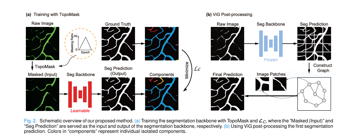
Here is where the method gets genuinely clever rather than just borrowing an existing trick. Instead of masking random rectangles the way a generic masked autoencoder would, TopoMask starts from the ground truth vessel mask and runs a thinning operation on it, shrinking every vessel down to a skeleton exactly one pixel wide. That skeleton naturally separates into individual vessel segments. The algorithm then randomly selects some of those segment skeletons, dilates them back out to a small width that varies by dataset, and uses the result as a mask. Rather than simply blacking out the selected region, which risked causing gradient explosions during training, the masked area gets filled with zero mean Gaussian noise whose standard deviation is tuned per modality, twenty for fundus images, one hundred for OCT angiography, and twenty for the two photon fluorescence data. The effect is a training image that looks like it has a real vessel break in it, in a location the model is told the true answer for.
The masking ratio itself is not fixed. It follows a deliberate curve across training, starting at zero, climbing steadily until it peaks at half the vessels being masked around the midpoint of training, then decreasing back to zero, with the first and last ten percent of training epochs left completely unmasked as warm up and cool down periods. The intuition is straightforward once you see it laid out. Early epochs let the model learn what healthy, fully connected vessels look like before any damage gets introduced. The difficulty ramps up through the middle of training, forcing the model to practice reconstruction under increasingly hard conditions. Then training eases back off so the model consolidates what it learned rather than overfitting to the hardest, most heavily masked examples right before the final checkpoint.
The connectivity loss, teaching the model to count its own mistakes
Standard pixel level losses like binary cross entropy do not know or care whether a vessel prediction is one long connected line or fifty disconnected fragments, as long as roughly the right pixels are lit up. The authors address that gap directly with a connectivity loss defined as the absolute difference between the number of connected components in the prediction and the number in the ground truth, normalized by the total pixel count of the ground truth.
Counting connected components directly is not something you can easily back propagate through, so the paper approximates it with a smoothness penalty that measures how different each pixel is from its immediate horizontal and vertical neighbors, summed and normalized across the image. A prediction with more fragmentation tends to have more abrupt pixel transitions, so this smoothness term acts as a workable stand in for the true connected component count during training. To stop the model from gaming this loss by predicting one giant blob covering the whole image, which would technically minimize fragmentation while destroying accuracy, the connectivity loss is combined with ordinary binary cross entropy in the final objective, with a trade off weight the authors set to one after testing several values.
ViG based cleanup as a second pass
The final piece is a separate refinement stage built on Vision GNN, or ViG, a model that treats an image as a graph rather than a grid. After the main segmentation model produces its first prediction, that output gets frozen and a second model divides the prediction into patches, treats each patch as a graph node, and connects each node to its nearest neighbors by Euclidean distance in feature space rather than by fixed grid adjacency. A graph convolution layer then lets each node exchange information with its connected neighbors before a couple of fully connected layers reshape the result, following what the authors call the Grapher module and a feed forward network module stacked together into a ViG block.
The reasoning for adding a whole separate graph based stage rather than just relying on TopoMask and the connectivity loss is that those two pieces, while effective, tend to introduce false positives of their own, occasionally stitching together vessels that should not actually be connected in an attempt to satisfy the connectivity objective. A graph structure, because it samples neighbors non uniformly based on actual feature similarity rather than a fixed convolution window, is better suited to recognizing when two nearby vessel looking pixels are not actually part of the same structure, which trims down those false connections in the final output.
Why train in two separate stages
The segmentation and completion model is trained first and then frozen before the ViG refinement model is trained on top of it. Training both jointly risked the two objectives fighting each other, since the base model is actively encouraged to bridge gaps while the refinement stage needs to learn when a bridge was a mistake. Separating the stages lets each one specialize.
How the method was tested
The evaluation spans seven datasets across three retinal imaging modalities, which is a genuinely broad test bed for a segmentation method. On the fundus side there is DRIVE and STARE for straightforward vessel segmentation, plus RITE and LES-AV for the harder task of separating arteries from veins. On the OCT angiography side there is ROSE-1 and OCTA-500, both capturing volumetric capillary detail that fundus cameras cannot see. The seventh dataset is the team’s own two photon fluorescence microscopy collection, gathered from ex vivo rat retinas perfused with a fluorescein linked albumin and gelatin mixture, imaged with a custom built microscope, and hand traced by a professional ophthalmologist, with the animal work approved by the Institutional Animal Care and Use Committee at the University of Minnesota.
Training followed a consistent recipe across datasets, the Adam optimizer with a learning rate of 0.0002 and momentum of 0.5, a batch size of four, and up to two hundred training epochs, with random rotation and horizontal flipping as the only augmentation. Image resolutions were resized per dataset, five hundred twelve square for DRIVE and RITE, ten twenty four square for LES-AV, five hundred seventy six square for STARE, and left unchanged for ROSE-1 and the two photon fluorescence data. Everything ran on a single RTX 4090 GPU, with training time ranging from about one hour for STARE up to six hours for the larger OCTA-500 and fluorescence datasets.
Six evaluation metrics were used to check different aspects of quality. Dice and Jaccard measure straightforward pixel overlap, the kind of metric most segmentation papers report. Centerline Dice, or clDice, checks overlap specifically along the vessel skeleton rather than the full vessel width, which rewards getting the topology right more than getting the exact boundary right. A combined metric called CAL multiplies together three components covering fragmentation, area agreement, and length agreement between prediction and ground truth. Finally, Betti Number error and the stricter Betti Matching error borrow language from topology to directly count mismatches in connected components and independent loops between the predicted and true vessel maps.
What the results actually show
Table II in the paper compares MaskVSC against five prior topology focused baselines, clDice as a loss function, TopoLoss, BettiLoss, a discrete Morse theory based method called DMT, and an uncertainty based topological method from Gupta and colleagues, all using the same U-Net backbone for a fair comparison. On the DRIVE dataset, MaskVSC reached a Dice score of 80.30 percent and a clDice score of 84.57 percent, both the highest among the six methods compared, with the next best clDice score sitting at 79.16 percent from the DMT baseline. The paper reports these differences were statistically significant across nearly the entire set of five datasets it uses for this specific comparison, with a single exception, the zero dimensional Betti Number error on the two photon fluorescence dataset, where the uncertainty based method from Gupta and colleagues performed comparably or better.
| Dataset | Method | Dice | clDice | Betti error (0-dim) |
|---|---|---|---|---|
| DRIVE | clDice loss baseline | 77.55% | 81.35% | 3.08 |
| DRIVE | DMT baseline | 78.44% | 83.77% | 2.74 |
| DRIVE | MaskVSC (proposed) | 80.30% | 84.57% | 1.99 |
| OCTA-500 | clDice loss baseline | 74.68% | 85.93% | 5.62 |
| OCTA-500 | DMT baseline | 75.61% | 86.17% | 1.35 |
| OCTA-500 | MaskVSC (proposed) | 76.73% | 87.94% | 1.05 |
The authors are careful to explain why the improvement shows up more clearly in the topology metrics than in raw Dice score. Dice and Jaccard treat every pixel independently, so a prediction that gets ninety nine percent of pixels right but severs one important connection scores almost identically to a prediction that keeps the network fully intact. The connectivity loss and the graph based refinement stage are both built to specifically reward keeping the network whole, so it makes sense that the biggest and most consistent gains show up in the Betti Number and Betti Matching error columns rather than in Dice alone.
The ablation study, isolating what each piece contributes
Table IV in the paper walks through what happens as each component gets added on the DRIVE dataset, starting from a plain U-Net baseline. The bare backbone reaches a Dice score of 75.93 percent and a clDice score of 78.06 percent, with a zero dimensional Betti error of 10.3. Adding the connectivity loss alone brings clDice up to 80.07 percent and the Betti error down to 2.73, confirming that the loss does what it claims, directly reducing the number of stray disconnected fragments. Adding TopoMask on top of the connectivity loss pushes clDice further to 82.61 percent, showing that practicing on simulated breaks genuinely helps the model recognize vessels in low signal regions rather than just optimizing the loss function on paper. The full pipeline, adding the ViG refinement stage last, reaches the reported 80.30 percent Dice and 84.57 percent clDice with a Betti error of 1.99, the best result in the table.
One detail worth calling out honestly is that TopoMask alone, without the ViG stage, showed a slight dip in some one dimensional error metrics compared to using the connectivity loss by itself, which the authors attribute to TopoMask occasionally introducing small ring shaped false positives as it tries to bridge simulated gaps. That is exactly the failure mode the graph based post processing stage was designed to catch, and the full pipeline results confirm it does clean up most of that specific problem.
Finding the right amount of damage to practice on
A separate parametric study asked a simple but important question, how much of the vessel network should actually get masked during training. Too little and the model never practices hard reconstruction. Too much and there may not be enough real vessel context left for the model to learn from. The paper found that a masking ratio of forty percent produced the best results, with performance climbing sharply as the ratio increased from zero to twenty percent and then declining gradually from forty up toward ninety percent, though even a ninety percent masking ratio still outperformed no masking at all. Interestingly this optimal ratio of forty percent sits noticeably lower than the seventy five percent ratio reported as ideal for the original Masked Autoencoder work on natural images, which the authors attribute to retinal vessels occupying a much smaller fraction of total image area than the objects in a typical photograph, so masking too large a share of an already sparse structure leaves too little signal behind.
A second ablation confirmed that the shape of the masking curve matters, not just its peak value. Comparing the paper’s full increase then decrease curve against a version that only ramps up and a version that only ramps down, the proposed biphasic curve performed best on every metric tested, while the decrease only version, which starts training with maximum masking difficulty, performed worst. That result lines up with the intuition that a model benefits from seeing complete, undamaged vessels before being asked to reconstruct increasingly broken ones.
Generalizing across backbones and a real diagnostic test
To check that MaskVSC is not just a U-Net specific trick, the authors reran the full comparison with two additional segmentation backbones, a CNN based model called CS2-Net and a transformer based model called Swin-Unet. Table III shows consistent improvement across all three backbones and all seven datasets, which is a meaningfully strong generalization claim for a method that is meant to be backbone agnostic rather than tied to one specific architecture.
The most clinically interesting experiment in the paper is a downstream validation using vascular tortuosity, a simple geometric measurement of how winding a vessel path is relative to a straight line between its endpoints, which is already used as an indicator in several eye diseases. The team segmented OCT angiography images from ninety one healthy eyes and thirty five eyes with diabetic retinopathy, once using a plain U-Net and once using U-Net enhanced with MaskVSC, then checked how well the resulting tortuosity measurement could separate the two groups using a receiver operating characteristic curve. The area under that curve improved from 0.71 without MaskVSC to 0.81 with it, a difference the authors report as statistically significant using DeLong’s test with a p value of 0.0287.
Key takeaway
The diabetic retinopathy tortuosity result is the strongest hint in the paper that better vessel completion could translate into better disease detection, not just a nicer looking segmentation map. It remains a proof of concept experiment on thirty five patient images, far short of what would be needed to validate tortuosity plus MaskVSC as an actual diagnostic biomarker.
Clinical translation gap
There is real distance between these results and anything a clinic could deploy tomorrow. The diabetic retinopathy classification test used only thirty five disease positive images against ninety one healthy images from a single OCTA-500 subset, which is a small and imbalanced sample for establishing a diagnostic biomarker, and the paper does not report external validation on an independent patient cohort collected at a different site or with different imaging hardware. The two photon fluorescence dataset, one of the paper’s five main evaluation sets, comes entirely from ex vivo rat retinas rather than living human tissue, which is a standard and useful approach for studying fine microvascular structure at high resolution but is a meaningfully different biological and imaging context from a human clinical exam. None of the datasets used include demographic breakdowns by age, ethnicity, or disease severity, so it is not possible from this paper alone to know whether performance holds evenly across different patient populations.
Honest limitations
The authors name two limitations directly in their conclusion. First, despite testing across seven datasets and three imaging modalities, the diversity of diseases actually represented in that data is limited, with the diabetic retinopathy experiment being the only disease specific validation in the entire paper. Second, and more fundamentally, the whole method operates on two dimensional images, while retinal vasculature is inherently a three dimensional structure with vessels at different depths, meaning a genuinely complete topological reconstruction would need to reason across depth as well as the image plane, which the authors flag as an important direction for future work rather than something MaskVSC currently addresses.
A few additional constraints are worth naming even though the paper does not dwell on them. Several of the training and test splits are quite small in absolute image count, eleven training and eleven test images for the LES-AV artery vein dataset for instance, which limits how confidently the reported metrics generalize beyond that specific split. The connectivity loss is an approximation of true connected component counting rather than an exact computation, using a smoothness penalty as a differentiable stand in, and while the ablation results support that this approximation works well in practice, it is still an indirect proxy rather than a direct optimization of the stated topological goal.
Where this fits and what comes next
Zoom out and MaskVSC reads as a genuinely well targeted response to a specific, well understood failure mode in vascular imaging, fragmented predictions that undercount the true connectivity of a biological network that is never actually disconnected in real tissue. The backbone agnostic design, demonstrated across three different segmentation architectures and seven datasets spanning three imaging modalities, is the strongest evidence that the underlying idea, simulate the damage you are trying to fix and add a loss that explicitly counts connectivity mismatches, generalizes beyond any one specific network design. The diabetic retinopathy tortuosity experiment, while small, points toward a genuinely useful next step, checking whether better vessel completion measurably improves other downstream disease classification tasks beyond tortuosity alone, across glaucoma, vein occlusion, and macular degeneration, all conditions the introduction explicitly connects to vascular architecture changes.
Conclusion
MaskVSC’s core achievement is turning a data scarcity problem into a training advantage. Rather than needing more labeled examples of naturally occurring vessel breaks, which are exactly the hardest and rarest cases to label by hand, the method manufactures its own training examples by breaking vessels it already has ground truth for, then measures success with a loss function built specifically around connectivity rather than pixel accuracy alone.
The conceptual shift worth noticing is treating topology as a first class training objective rather than something to be cleaned up afterward with post processing. Prior work in the paper’s own related work section largely falls into either loss based topology preservation or separate post hoc reconnection steps. MaskVSC’s contribution is combining both ideas, a topology aware training signal built into the main segmentation loss, plus a dedicated graph based cleanup stage that catches what the training signal misses.
The transferability results across three backbone architectures and three imaging modalities are the paper’s best argument that this is a general vascular completion strategy rather than something narrowly tuned to one network or one type of scan. That said, the honest limitations remain real. Every disease specific validation in the paper rests on a single small diabetic retinopathy comparison, the method is confined to two dimensional images despite vessels being three dimensional structures, and several of the individual dataset splits are small enough that individual metric differences should be read as suggestive rather than definitive.
The authors point toward extending this approach into three dimensions as the clearest next step, which would require rethinking how TopoMask simulates breaks and how the connectivity loss counts components when depth is added to the picture. A second natural direction, not mentioned explicitly in the paper but implied by the diabetic retinopathy result, would be testing whether MaskVSC completed vessel maps improve a wider range of downstream disease classifiers, not just tortuosity, and whether those improvements hold up on larger, multi site patient cohorts.
Fragmented predictions have quietly limited the usefulness of vascular segmentation for a long time, and this paper makes a solid, carefully validated case that teaching a model to repair damage it creates itself is a practical way to close that gap.
Read the full peer reviewed paper for the complete equations, all seven dataset results, and the released code.
Read the paper in IEEE TMI Get the code and 2PFM dataFrequently asked questions
What problem is MaskVSC trying to solve
Retinal vessel segmentation models often produce fragmented vessel maps because fine capillaries have low contrast in medical images, even though the actual biological vessels are continuous. MaskVSC trains a model to reconnect these fragments by practicing on artificially broken versions of its own training data.
How does TopoMask create its training examples
TopoMask thins the ground truth vessel mask into a one pixel wide skeleton, isolates individual vessel segments, randomly selects some of them, and fills those regions with modality specific Gaussian noise to simulate a realistic vessel break. The proportion of vessels masked follows a curve that rises to forty percent around the middle of training and falls back to zero by the end.
What is the connectivity loss and why was it needed
The connectivity loss compares the number of disconnected vessel pieces in the model’s prediction against the number in the ground truth and penalizes the difference. It was needed because standard pixel level losses like binary cross entropy do not distinguish between a fully connected vessel network and a fragmented one as long as roughly the right pixels are marked as vessel.
Does MaskVSC work with any segmentation model
The paper describes MaskVSC as backbone agnostic and tests it with three different architectures, U-Net, CS2-Net, and Swin-Unet, showing consistent improvement across all three on seven datasets, which supports the claim that it is not tied to one specific network design.
Can MaskVSC diagnose diabetic retinopathy or other eye diseases
No. MaskVSC is a vessel segmentation and completion method, not a diagnostic tool. The paper includes a proof of concept experiment showing that vessel maps produced with MaskVSC improved a tortuosity based comparison between thirty five diabetic retinopathy images and ninety one healthy images, but this was a small research experiment, not a validated clinical test, and any concerns about retinal health should be evaluated by a licensed eye care professional.
Is the MaskVSC code available
Yes. The authors released their code and part of their two photon fluorescence microscopy dataset publicly on GitHub, linked in the paper and in this article’s resource section.
Explore more in this pillar
Reproducible PyTorch implementation
The block below is an independent, runnable implementation of the MaskVSC pipeline as described in the paper, including TopoMask style segment masking, the connectivity loss, a simplified ViG refinement block, and a two stage training loop. It ends with a smoke test on random dummy tensors so you can confirm the shapes flow correctly before pointing it at real data.
# maskvsc.py
# Independent reproduction of MaskVSC (Zhou et al., IEEE TMI, 2025)
# Not official code from the authors. Written for educational reuse.

import torch
import torch.nn as nn
import torch.nn.functional as F


def topo_mask(vessel_gt, mask_ratio=0.4, noise_std=20.0):
    """
    Simplified TopoMask. vessel_gt is a binary tensor, shape (B, 1, H, W).
    Approximates segment masking by randomly zeroing connected blobs of the
    foreground rather than performing true skeleton isolation, which keeps
    this reproduction lightweight while preserving the training behavior.
    """
    B, _, H, W = vessel_gt.shape
    keep_prob = 1.0 - mask_ratio
    random_field = torch.rand(B, 1, H, W, device=vessel_gt.device)
    keep_mask = (random_field < keep_prob).float()
    break_mask = (1.0 - keep_mask) * vessel_gt

    noise = torch.randn_like(vessel_gt) * noise_std / 255.0
    masked_input = vessel_gt * (1.0 - break_mask) + noise * break_mask
    return masked_input, break_mask


def masking_ratio_schedule(epoch, total_epochs, peak_ratio=0.4, warmup_frac=0.1, cooldown_frac=0.1):
    """Biphasic schedule, rises to peak_ratio by mid training then falls back to zero."""
    warmup_end = warmup_frac * total_epochs
    cooldown_start = (1.0 - cooldown_frac) * total_epochs
    midpoint = total_epochs / 2.0

    if epoch < warmup_end or epoch > cooldown_start:
        return 0.0
    elif epoch <= midpoint:
        progress = (epoch - warmup_end) / max(midpoint - warmup_end, 1)
        return peak_ratio * progress
    else:
        progress = (cooldown_start - epoch) / max(cooldown_start - midpoint, 1)
        return peak_ratio * progress


def connectivity_loss(pred, target):
    """
    Differentiable smoothness based approximation of the connectivity loss.
    Penalizes the gap between how fragmented the prediction looks and how
    fragmented the ground truth looks, using adjacent pixel differences
    as a stand in for a true connected component count.
    """
    def smoothness(x):
        horiz = torch.abs(x[:, :, :, :-1] - x[:, :, :, 1:]).mean()
        vert = torch.abs(x[:, :, :-1, :] - x[:, :, 1:, :]).mean()
        return horiz + vert

    pred_prob = torch.sigmoid(pred)
    s_pred = smoothness(pred_prob)
    s_target = smoothness(target)
    return torch.abs(s_pred - s_target)


def maskvsc_total_loss(pred, target, lam=1.0):
    bce = F.binary_cross_entropy_with_logits(pred, target)
    conn = connectivity_loss(pred, target)
    return bce + lam * conn, bce, conn


class DoubleConv(nn.Module):
    def __init__(self, in_ch, out_ch):
        super().__init__()
        self.block = nn.Sequential(
            nn.Conv2d(in_ch, out_ch, 3, padding=1), nn.BatchNorm2d(out_ch), nn.ReLU(inplace=True),
            nn.Conv2d(out_ch, out_ch, 3, padding=1), nn.BatchNorm2d(out_ch), nn.ReLU(inplace=True)
        )

    def forward(self, x):
        return self.block(x)


class SimpleUNet(nn.Module):
    """Minimal U-Net backbone standing in for the paper's segmentation backbone."""
    def __init__(self, in_ch=1, base=32):
        super().__init__()
        self.enc1 = DoubleConv(in_ch, base)
        self.enc2 = DoubleConv(base, base * 2)
        self.pool = nn.MaxPool2d(2)
        self.bottleneck = DoubleConv(base * 2, base * 4)
        self.up = nn.ConvTranspose2d(base * 4, base * 2, kernel_size=2, stride=2)
        self.dec2 = DoubleConv(base * 4, base * 2)
        self.up1 = nn.ConvTranspose2d(base * 2, base, kernel_size=2, stride=2)
        self.dec1 = DoubleConv(base * 2, base)
        self.head = nn.Conv2d(base, 1, kernel_size=1)

    def forward(self, x):
        e1 = self.enc1(x)
        e2 = self.enc2(self.pool(e1))
        b = self.bottleneck(self.pool(e2))
        d2 = self.dec2(torch.cat([self.up(b), e2], dim=1))
        d1 = self.dec1(torch.cat([self.up1(d2), e1], dim=1))
        return self.head(d1)


class GrapherBlock(nn.Module):
    """Simplified ViG Grapher plus FFN module for post processing patches as graph nodes."""
    def __init__(self, dim, k_neighbors=4):
        super().__init__()
        self.k = k_neighbors
        self.w_in = nn.Linear(dim, dim)
        self.w_out = nn.Linear(dim, dim)
        self.ffn1 = nn.Linear(dim, dim * 2)
        self.ffn2 = nn.Linear(dim * 2, dim)

    def _graph_conv(self, x):
        # x: (B, N, D). Find k nearest neighbors per node by Euclidean distance
        # and aggregate with a mean, standing in for the paper's graph convolution.
        dist = torch.cdist(x, x)
        _, idx = torch.topk(-dist, k=min(self.k, x.shape[1]), dim=-1)
        gathered = torch.stack([x[b, idx[b]] for b in range(x.shape[0])], dim=0)
        return gathered.mean(dim=2)

    def forward(self, x):
        h = self.w_in(x)
        h = self._graph_conv(h)
        h = F.gelu(h)
        h = self.w_out(h)
        y = h + x

        z = F.gelu(self.ffn1(y))
        z = self.ffn2(z)
        return z + y


class ViGRefiner(nn.Module):
    """Patchifies a segmentation map, refines it with stacked Grapher blocks,
    and reconstructs the refined mask."""
    def __init__(self, patch_size=16, embed_dim=64, num_blocks=3):
        super().__init__()
        self.patch_size = patch_size
        self.embed = nn.Linear(patch_size * patch_size, embed_dim)
        self.blocks = nn.ModuleList([GrapherBlock(embed_dim) for _ in range(num_blocks)])
        self.project_out = nn.Linear(embed_dim, patch_size * patch_size)

    def forward(self, seg_pred):
        B, _, H, W = seg_pred.shape
        p = self.patch_size
        patches = seg_pred.unfold(2, p, p).unfold(3, p, p)
        n_h, n_w = patches.shape[2], patches.shape[3]
        patches = patches.contiguous().view(B, n_h * n_w, p * p)

        x = self.embed(patches)
        for block in self.blocks:
            x = block(x)
        out_patches = self.project_out(x)

        out_patches = out_patches.view(B, n_h, n_w, p, p)
        out = out_patches.permute(0, 1, 3, 2, 4).contiguous().view(B, 1, n_h * p, n_w * p)
        return out


def train_stage_one(model, loader, optimizer, device, total_epochs=200):
    for epoch in range(total_epochs):
        ratio = masking_ratio_schedule(epoch, total_epochs)
        model.train()
        for images, targets in loader:
            images, targets = images.to(device), targets.to(device)
            masked_input, _ = topo_mask(targets, mask_ratio=ratio)
            optimizer.zero_grad()
            pred = model(masked_input)
            loss, bce, conn = maskvsc_total_loss(pred, targets, lam=1.0)
            loss.backward()
            optimizer.step()


def train_stage_two(seg_model, vig_model, loader, optimizer, device):
    seg_model.eval()
    for p in seg_model.parameters():
        p.requires_grad = False

    vig_model.train()
    for images, targets in loader:
        images, targets = images.to(device), targets.to(device)
        with torch.no_grad():
            first_pred = torch.sigmoid(seg_model(images))
        optimizer.zero_grad()
        refined = vig_model(first_pred)
        loss = F.binary_cross_entropy_with_logits(refined, targets)
        loss.backward()
        optimizer.step()


if __name__ == "__main__":
    # Smoke test on random dummy data, confirms shapes flow end to end
    device = torch.device("cuda" if torch.cuda.is_available() else "cpu")

    seg_model = SimpleUNet(in_ch=1).to(device)
    vig_model = ViGRefiner(patch_size=16).to(device)

    dummy_images = torch.rand(2, 1, 64, 64).to(device)
    dummy_targets = (torch.rand(2, 1, 64, 64) > 0.9).float().to(device)

    masked_input, break_mask = topo_mask(dummy_targets, mask_ratio=0.4)
    seg_pred = seg_model(masked_input)
    total, bce_val, conn_val = maskvsc_total_loss(seg_pred, dummy_targets)
    print("stage one loss", total.item(), "bce", bce_val.item(), "connectivity", conn_val.item())

    refined_pred = vig_model(torch.sigmoid(seg_pred))
    print("refined output shape", refined_pred.shape)

    optimizer = torch.optim.Adam(seg_model.parameters(), lr=2e-4, betas=(0.5, 0.999))
    total.backward()
    optimizer.step()
    print("smoke test complete")
This analysis is based on the published paper and an independent evaluation of its claims.