
Key Points
- Researchers turned whole slide pathology images into graphs, with each node representing an image patch and each edge representing physical adjacency between patches.
- A graph attention mechanism lets each patch learn from its neighboring tissue regions, and a second attention module fuses that spatial information with gene expression signatures tied to B cell immune activity.
- Tested on non small cell lung cancer cases from TCGA and CPTAC, the fusion model beat six published multimodal survival methods on most, though not all, comparison columns.
- The imaging only version of the model, without any genomic data, still outperformed every prior imaging only method the authors compared against.
- The model produces survival activation maps that highlight which tissue regions drove its prediction, and these maps overlapped meaningfully with a pathologist’s manual tumor annotations on a small held out set of slides.
- Published in IEEE Transactions on Medical Imaging in September 2024, this work has completed peer review, which sets it apart from many preprints covered on this site.
The problem with fusing images and genes late in the pipeline
Predicting how a cancer patient’s disease will progress from a combination of pathology images and molecular data is a well established goal in computational pathology. The typical approach processes the whole slide image through one pipeline, processes the gene expression data through a separate pipeline, and then merges the two outputs near the very end, an approach researchers call late fusion. A widely used method in this category, developed by Chen and colleagues, applies this weakly supervised late fusion strategy across many cancer types with real success.
The Boston University team, led by Yi Zheng and senior authors Jennifer Beane and Vijaya Kolachalama, argue that late fusion has a structural limitation. Gene expression data does not have an obvious spatial location the way an image does. A given gene signature does not point to a specific patch of tissue on its own. Late fusion combines the two data types only after each has already been distilled into a single summary vector, which means the model never gets the chance to learn which specific regions of the tumor a particular gene signature is actually associated with. The authors wanted a framework that learns those spatial relationships during training rather than discovering them, if at all, only through post hoc interpretation.
Why lung cancer and why B cell signatures
The team focused on non small cell lung cancer, which includes two major subtypes, lung adenocarcinoma and lung squamous cell carcinoma, denoted LUAD and LUSC. These are the two most common histological forms of non small cell lung cancer and together represent a large share of lung cancer diagnoses. For the genomic side, the authors chose five gene expression signatures tied to B cell immune populations, derived from prior single cell RNA sequencing studies of lung tissue. B cell related signatures are elevated in both LUAD and LUSC tumors, but the paper notes a genuinely interesting biological wrinkle, elevated tumor infiltrating B cells are associated with a better prognosis only in LUAD, not consistently in LUSC. That existing biological knowledge gave the team a meaningful test case, a scenario where a model that actually learns spatial gene image relationships should be able to pick up on a real, previously documented immunological pattern rather than a coincidental one.
How the graph based fusion actually works
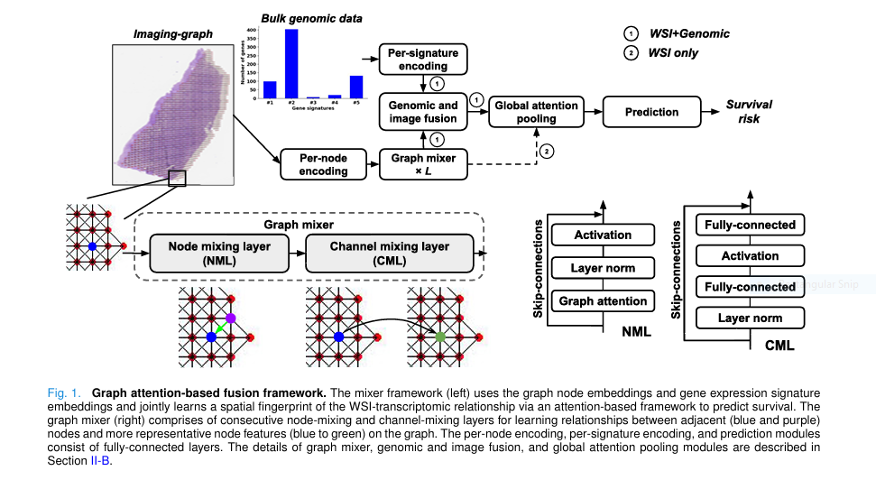
The architecture has several connected stages, moving from raw image pixels to a single survival risk estimate.
Turning a slide into a graph
A whole slide image is first separated from its background, then tessellated into a grid of small image patches. Each patch becomes a node in an undirected graph, and an edge connects two nodes if their patches are physically adjacent on the slide, with each patch allowed up to eight neighbors to capture full diagonal and orthogonal adjacency. Every node gets an initial feature vector by passing its patch through a convolutional encoder that was pretrained using contrastive learning, a self supervised technique where the network learns to recognize that different augmented crops of the same patch should produce similar embeddings while crops from different patches should not. This encoder was fine tuned specifically on the National Lung Screening Trial imaging data before being used to featurize the TCGA and CPTAC slides.
The graph mixer, learning from neighboring tissue
Once the slide is a graph, the model processes it through a stack of what the authors call GraphMixer layers, inspired by the MLP Mixer architecture originally built for standard image grids but adapted here to handle graphs with a variable number of nodes. Each GraphMixer layer has two parts, a node mixing layer that lets each patch attend to its immediate neighbors using a graph attention mechanism, and a channel mixing layer that processes the feature dimensions of each patch independently, similar to the channel mixing step in the original MLP Mixer.
The graph attention step, built on the Graph Attention Network architecture, computes a learned importance score between each patch and its neighbors rather than treating every neighboring patch as equally informative, which is what a simpler graph convolutional network would do.
Node \(i\) computes an attention weighted average of its neighbors \(N_i\), letting the network decide which adjacent tissue patches matter more for this particular node’s updated representation.
Bringing gene expression into the picture
After three GraphMixer layers refine the patch level representations, the model introduces the gene expression data through what the authors call the Genomic Attention Module. Each of the five gene signatures gets its own trainable encoder that turns it into a fixed length embedding. The module then applies a query key value attention mechanism, the same core idea behind transformer attention, where the gene signature embeddings act as queries that search across all the image patch embeddings to find which tissue regions are most relevant to that particular signature.
Here \(B\) holds the gene signature embeddings and \(H\) holds the patch embeddings after graph mixing, so the attention weights explicitly connect a molecular signature to specific spatial regions of the tumor.
This is the mechanism that lets the model learn, for instance, that a particular B cell signature tends to associate with a specific histologic pattern in a specific region of a slide, rather than simply averaging the whole slide’s imaging features with a global genomic summary vector the way late fusion approaches typically do.
From patch attention to one risk number
The fused patch level features then pass through a global attention pooling layer, a gated attention mechanism adapted from a widely used multiple instance learning framework, which produces a single slide level embedding while automatically weighting the more prognostically important patches more heavily. That final embedding feeds into a survival model built around a discrete time framework, where continuous survival time is split into four bins based on the quartiles of observed event times in the training cohort, and the model predicts a hazard probability for each bin. The loss function combines separate terms for patients whose death or progression was actually observed, called uncensored cases, and patients who were still alive or lost to follow up at the end of the study window, called censored cases, since those two groups carry different kinds of statistical information about survival time.
The team built two versions of this system. The imaging survival model, ISM, uses only the whole slide graph and skips the genomic attention step entirely. The fusion survival model, FSM, adds the Genomic Attention Module and the five B cell gene signatures on top. Comparing these two head to head is how the paper isolates how much the genomic data actually contributes on top of imaging alone.
The data behind the numbers
The study drew on three separate cohorts, each playing a distinct role. TCGA, The Cancer Genome Atlas, provided 444 LUAD and 471 LUSC cases used for training the survival models with five fold cross validation. CPTAC, the Clinical Proteomic Tumor Analysis Consortium, provided a separate 199 LUAD and 102 LUSC cases used purely as an independent external test set, meaning the models never saw this data during training or tuning. NLST, the National Lung Screening Trial, contributed imaging data used only to fine tune the contrastive learning feature extractor, not for survival label training. Keeping these three roles distinct is a meaningful methodological choice, since it means the reported CPTAC results reflect genuine generalization to an external cohort rather than performance on a held out split of the same source data.
Gene count data for both cohorts went through a careful preprocessing pipeline, filtering out duplicate samples and low signal genes, computing normalized expression values, and applying batch correction to align the CPTAC and TCGA gene expression scales, with TCGA serving as the reference batch. The final analysis used a common set of over twelve thousand genes shared across both LUAD and LUSC datasets after this cleanup.
What the results show, including where the fusion model does not win
The imaging only ISM model outperformed every other imaging only method the authors tested on the TCGA training cohort, reaching a concordance index of 0.687 for LUAD and 0.652 for LUSC, ahead of transformer based approaches like TransMIL and graph based approaches like Patch GCN. Concordance index, or c-index, measures how well a model ranks patients by relative survival risk, where 0.5 represents random guessing and 1.0 represents perfect ranking.
| Method | TCGA LUAD | TCGA LUSC | CPTAC LUAD | CPTAC LUSC |
|---|---|---|---|---|
| Attention MIL | 0.629 | 0.618 | 0.508 | 0.550 |
| Patch GCN | 0.645 | 0.650 | 0.558 | 0.536 |
| DeepAttnMISL | 0.671 | 0.624 | 0.515 | 0.557 |
| PathomicFusion | 0.662 | 0.620 | 0.515 | 0.568 |
| MCAT | 0.682 | 0.640 | 0.581 | 0.546 |
| PORPOISE | 0.688 | 0.619 | 0.506 | 0.562 |
| MOTCAT | 0.692 | 0.651 | 0.558 | 0.593 |
| FSM (this paper) | 0.703 | 0.664 | 0.579 | 0.678 |
Look at the CPTAC LUAD column closely. MCAT, a co attention based fusion method published in 2021, actually edges out FSM there, 0.581 against 0.579, a difference small enough to fall well within typical fold to fold variability but real in the reported numbers nonetheless. The paper’s own bold and dagger notation in its results table acknowledges this, marking MCAT as the best performer for that specific column while FSM leads everywhere else. That is a useful reminder that a model billed as state of the art rarely wins every single comparison cell in a results table, and CPTAC LUAD, the smallest of the four test columns at 199 cases, is exactly where fold to fold noise would be expected to matter most.
The time dependent area under the curve, or tAUC, tells a similar story with an even more pronounced exception. This metric evaluates how well the model separates high and low risk patients specifically at different points in time, rather than as a single ranking across the whole follow up period.
| Method | TCGA LUAD | TCGA LUSC | CPTAC LUAD | CPTAC LUSC |
|---|---|---|---|---|
| MCAT | 0.605 | 0.711 | 0.623 | 0.769 |
| PORPOISE | 0.592 | 0.648 | 0.541 | 0.648 |
| MOTCAT | 0.635 | 0.677 | 0.610 | 0.683 |
| FSM (this paper) | 0.679 | 0.681 | 0.613 | 0.792 |
Here MCAT beats FSM on two of the four columns, TCGA LUSC by a meaningful margin, 0.711 against 0.681, and CPTAC LUAD by a smaller one, 0.623 against 0.613. FSM’s advantage is concentrated in the LUAD TCGA column and the LUSC CPTAC column, where it wins clearly. Put plainly, if you cared specifically about how well a model ranks LUSC patients over time on the TCGA training distribution, MCAT’s co attention approach was the stronger published method in this particular study, not the graph based fusion approach this paper introduces. The overall pattern across both tables still favors FSM more often than not, and the CPTAC LUSC tAUC result, 0.792, is a clear and substantial win, but a fair reading of this paper does not describe FSM as sweeping every benchmark.
The authors offer a specific and testable explanation for this pattern rather than a vague one. TCGA’s recorded survival times span a much wider range, up to 7,143 days for LUAD, while CPTAC’s survival times cap out much lower, around 1,836 days for LUAD. Because CPTAC’s follow up window is shorter, almost all of its cases look like high risk cases relative to the TCGA derived risk thresholds the model was trained on, which compresses the ranking signal that c-index depends on even though the model’s underlying time dependent true positive and false positive rates, captured by tAUC, remain reasonably intact. That is a genuinely useful methodological insight for anyone building survival models across cohorts with different follow up durations, and it is stated plainly in the paper rather than glossed over.
What the ablation study adds beyond the headline numbers
The authors ran a detailed ablation study on the TCGA cohort, systematically swapping out individual components of the architecture. Four findings stand out as genuinely informative for anyone considering a similar design.
| Configuration | LUAD | LUSC |
|---|---|---|
| Full model, contrastive ResNet18 features, node and channel mixing, genomic attention | 0.703 | 0.664 |
| Same but with ImageNet pretrained features instead of contrastive features | 0.661 | 0.638 |
| Node mixing layer only, no channel mixing, no genomic attention | 0.654 | 0.607 |
| Channel mixing layer only, no node mixing, no genomic attention | 0.589 | 0.532 |
| Graph convolutional network instead of graph attention, with genomic attention | 0.685 | 0.647 |
| Contrastive ResNet50 features instead of ResNet18, no genomic attention | 0.679 | 0.642 |
| Four neighbor connectivity instead of eight, with genomic attention | 0.691 | 0.648 |
The node mixing layer, the part responsible for letting patches learn from their spatial neighbors, matters far more on its own than the channel mixing layer does, 0.654 against 0.589 on LUAD when each is used without the other. Contrastive self supervised features beat ImageNet pretrained features by a clear margin, 0.703 against 0.661, which fits the general pattern in computational pathology that domain specific self supervised pretraining tends to outperform generic natural image pretraining. A detail the abstract does not mention at all, moving from a ResNet18 to a larger ResNet50 backbone for the contrastive feature extractor did not help and in fact slightly hurt performance, which the authors attribute to the limited size of the NLST dataset used for that particular self supervised fine tuning step, not enough data to fully exploit a larger backbone’s extra capacity. Graph attention edged out a simpler graph convolutional network, 0.703 against 0.685, though the gap here is smaller than some of the other ablation swaps, meaning the choice of attention over convolution mattered less than the choice of contrastive over ImageNet features or the inclusion of node mixing at all.
How the model explains its own predictions
Beyond raw performance metrics, the paper introduces survival activation maps, an adaptation of the Grad-CAM technique that highlights which regions of a slide most influenced the model’s risk prediction. Grad-CAM was originally built for standard convolutional networks and does not directly apply to a graph based architecture without convolutional layers, so the authors adapted it to work with gradients flowing back to the graph mixer’s node features instead.
To check whether these maps actually mean something clinically, the team had a pathologist manually annotate ten whole slide images from the CPTAC cohort, marking tumor regions by histologic pattern, including patterns known from the literature to carry prognostic significance, such as the aggressive solid growth pattern versus the more favorable lepidic pattern in lung adenocarcinoma, and separately marking evidence of vascular invasion. Comparing the model’s survival activation maps against these expert annotations using the Dice coefficient, a standard measure of spatial overlap, showed that the fusion model’s maps aligned more closely with pathologist annotations than either a simpler attention based heatmap or the co attention weights from the genomic fusion step alone. In one case, the fusion model specifically highlighted the aggressive solid tumor pattern and a documented focus of vascular invasion, both patterns independently associated with worse prognosis in the existing pathology literature, which is a meaningfully specific and checkable form of validation rather than a vague claim of interpretability.
The clinical translation gap
This paper clears a bar that a lot of computational pathology research does not, it has completed formal peer review and appeared in a well established imaging journal, and it tests its model on a genuinely external cohort, CPTAC, rather than only on held out splits of the same source data. That is meaningfully more rigorous than many preprints. Even so, there is real distance between what this study demonstrates and a tool ready for clinical decision making.
The survival models here were trained and tested entirely on retrospective, deidentified research cohort data, not on a prospective clinical workflow where a prediction would actually inform a treatment decision in real time. The gene expression data used is bulk RNA sequencing from resected tumor tissue, a laboratory process not currently part of routine clinical care for most lung cancer patients, so even a clinically validated version of this fusion approach would require gene expression profiling infrastructure most hospitals do not have as standard practice today. The five gene signatures tested are specific to B cell immune populations, chosen as what the authors themselves describe as a proof of concept, and the paper does not claim these particular signatures are the optimal or final choice for prognostic gene fusion, only that the fusion mechanism itself can learn something meaningful from them.
Perhaps most importantly, a c-index around 0.65 to 0.70, while a genuine improvement over prior published methods, still reflects a moderate rather than a highly precise ability to rank individual patients by survival risk. A c-index of 1.0 would represent perfect discrimination and 0.5 represents no better than chance, so these results sit meaningfully above chance but well short of a level of precision that would support individual level clinical decisions on their own, separate from a full clinical workup.
Honest limitations
The authors are notably candid about several limitations in their own discussion section, and it is worth naming them directly rather than only summarizing the strengths.
The pathologist annotation comparison used only ten CPTAC cases, explicitly because manual annotation is time consuming and pathologist availability was limited for the study. Conclusions about how well the survival activation maps match real prognostic tissue features rest on this small sample and the authors describe their own conclusions here as limited for that reason.
The survival loss function relies on a proportional hazards style assumption embedded in its likelihood formulation. If the true relationship between risk factors and survival time does not hold this assumption, meaning hazard ratios that are not actually constant over time, the model’s risk estimates could become biased in ways that are hard to detect from aggregate metrics like c-index alone.
Censoring, the statistical reality that many patients in a survival study are still alive or lost to follow up when the study ends, complicates model training in ways the authors flag as an open challenge. Datasets with very different censoring rates, which is exactly the situation between TCGA and CPTAC in this study, can produce systematically different quality of survival time estimates, and the authors suggest inverse probability of censoring weighting as a promising but untested direction for future work rather than something they have already solved.
The CPTAC c-index drop discussed earlier, while explained by a plausible follow up window mismatch, still represents a real and measurable degradation in one of the two headline metrics when the model moved from its training distribution to an external cohort, a pattern worth remembering any time a paper reports strong internal cross validation numbers alongside separately reported external test numbers.
Finally, the five B cell gene signatures tested represent one biologically motivated but narrow slice of what tumor gene expression actually contains. The paper explicitly frames this as a proof of concept and states that testing other cell type and prognostic gene signature sets is planned future work, not something this particular study has already validated.
Where this fits into the bigger picture
The broader trend this paper belongs to is the move from late fusion, where imaging and non imaging data meet only at the very end of a pipeline, toward early and mid level fusion, where different data modalities influence each other’s representations throughout training. That shift matters for any diagnostic or prognostic task where a non imaging biomarker plausibly has some meaningful spatial relationship to tissue architecture, not just lung cancer prognosis specifically. The graph representation of whole slide images, with attention based node mixing, is also a reusable idea independent of the survival prediction task itself, and the authors note their genomic data, code, and trained model scripts are publicly available on GitHub, which lowers the barrier for other groups to test the same fusion mechanism against different cancer types or different molecular data types such as proteomics or spatial transcriptomics.
Complete PyTorch implementation
Below is a runnable implementation of the core architecture described above, a graph attention based node mixing layer, a channel mixing layer combined into a GraphMixer block, the Genomic Attention Module for fusing gene signature embeddings with patch embeddings, gated global attention pooling, and the discrete time survival loss with separate censored and uncensored terms. A smoke test at the bottom runs the full pipeline on random dummy data to confirm the shapes and the backward pass work end to end.
import torch
import torch.nn as nn
import torch.nn.functional as F

# ----------------------------------------------------------------------
# Graph attention layer used inside the Node Mixing Layer (NML)
# ----------------------------------------------------------------------
class GraphAttentionLayer(nn.Module):
    def __init__(self, dim):
        super().__init__()
        self.W = nn.Linear(dim, dim, bias=False)
        self.a = nn.Parameter(torch.empty(2 * dim, 1))
        nn.init.xavier_uniform_(self.a)
        self.leaky_relu = nn.LeakyReLU(0.2)

    def forward(self, h, adjacency):
        # h: N,D node features. adjacency: N,N binary matrix.
        n = h.shape[0]
        wh = self.W(h)
        wh_i = wh.unsqueeze(1).expand(n, n, -1)
        wh_j = wh.unsqueeze(0).expand(n, n, -1)
        concat = torch.cat([wh_i, wh_j], dim=-1)
        e = self.leaky_relu((concat @ self.a).squeeze(-1))

        # mask out non-neighbors before softmax
        neg_inf = torch.finfo(e.dtype).min
        e_masked = torch.where(adjacency > 0, e, torch.full_like(e, neg_inf))
        attn = F.softmax(e_masked, dim=1)
        h_new = torch.matmul(attn, wh)
        return F.elu(h_new)


# ----------------------------------------------------------------------
# GraphMixer block, node mixing (graph attention) then channel mixing
# ----------------------------------------------------------------------
class ChannelMixingLayer(nn.Module):
    def __init__(self, dim, hidden_mult=2):
        super().__init__()
        self.net = nn.Sequential(
            nn.Linear(dim, dim * hidden_mult),
            nn.GELU(),
            nn.Linear(dim * hidden_mult, dim)
        )

    def forward(self, h):
        return self.net(h)


class GraphMixerLayer(nn.Module):
    def __init__(self, dim):
        super().__init__()
        self.ln1 = nn.LayerNorm(dim)
        self.gat = GraphAttentionLayer(dim)
        self.nml_out = nn.Linear(dim, dim)
        self.ln2 = nn.LayerNorm(dim)
        self.cml = ChannelMixingLayer(dim)

    def forward(self, h, adjacency):
        h_prime = h + self.nml_out(self.gat(self.ln1(h), adjacency))
        h_out = h_prime + self.cml(self.ln2(h_prime))
        return h_out


# ----------------------------------------------------------------------
# Genomic Attention Module (GAM), fuses gene signature embeddings with
# patch embeddings via query key value attention
# ----------------------------------------------------------------------
class GenomicAttentionModule(nn.Module):
    def __init__(self, dim):
        super().__init__()
        self.wq = nn.Linear(dim, dim, bias=False)
        self.wk = nn.Linear(dim, dim, bias=False)
        self.wv = nn.Linear(dim, dim, bias=False)
        self.scale = dim ** 0.5

    def forward(self, gene_embeddings, node_embeddings):
        # gene_embeddings: M,D   node_embeddings: N,D
        q = self.wq(gene_embeddings)
        k = self.wk(node_embeddings)
        v = self.wv(node_embeddings)
        attn = F.softmax((q @ k.transpose(0, 1)) / self.scale, dim=-1)
        return attn @ v  # M,D fused genomic-image embeddings


# ----------------------------------------------------------------------
# Gated global attention pooling over graph nodes
# ----------------------------------------------------------------------
class GatedAttentionPooling(nn.Module):
    def __init__(self, dim, hidden=128):
        super().__init__()
        self.v = nn.Linear(dim, hidden, bias=False)
        self.u = nn.Linear(dim, hidden, bias=False)
        self.w = nn.Linear(hidden, 1, bias=False)

    def forward(self, h):
        gate = torch.tanh(self.v(h)) * torch.sigmoid(self.u(h))
        scores = self.w(gate).squeeze(-1)
        weights = F.softmax(scores, dim=0)
        pooled = (weights.unsqueeze(-1) * h).sum(dim=0)
        return pooled, weights


# ----------------------------------------------------------------------
# Discrete time survival loss, separate censored and uncensored terms
# ----------------------------------------------------------------------
def survival_loss(hazard_logits, discrete_time, is_censored, alpha=0.5):
    # hazard_logits: num_bins raw scores for one patient
    # discrete_time: integer bin index for this patient's event or censor time
    # is_censored: 1.0 if censored, 0.0 if event observed
    hazard = torch.sigmoid(hazard_logits)
    survival = torch.cumprod(1.0 - hazard, dim=0)

    y = discrete_time
    s_prev = survival[y - 1] if y > 0 else torch.tensor(1.0)
    h_y = hazard[y]
    s_y = survival[y]

    if is_censored < 0.5:
        # uncensored, event actually observed at bin y
        loss = -torch.log(s_prev + 1e-8) - torch.log(h_y + 1e-8)
    else:
        # censored, only know the patient survived at least to bin y
        loss = -torch.log(s_y + 1e-8)
    return loss


def batch_survival_loss(hazard_logits_batch, times, censored_flags, alpha=0.5, beta=0.5):
    losses = []
    for logits, t, c in zip(hazard_logits_batch, times, censored_flags):
        losses.append(survival_loss(logits, t, c))
    return torch.stack(losses).mean()


# ----------------------------------------------------------------------
# Full fusion survival model wrapper
# ----------------------------------------------------------------------
class FusionSurvivalModel(nn.Module):
    def __init__(self, patch_feat_dim, hidden_dim=64, num_layers=3,
                 num_signatures=5, num_bins=4):
        super().__init__()
        self.node_embed = nn.Linear(patch_feat_dim, hidden_dim)
        self.mixer_layers = nn.ModuleList(
            [GraphMixerLayer(hidden_dim) for _ in range(num_layers)]
        )
        self.signature_encoders = nn.ModuleList(
            [nn.Linear(1, hidden_dim) for _ in range(num_signatures)]
        )
        self.gam = GenomicAttentionModule(hidden_dim)
        self.pool = GatedAttentionPooling(hidden_dim)
        self.hazard_head = nn.Linear(hidden_dim, num_bins)

    def forward(self, patch_features, adjacency, gene_signature_scores):
        # patch_features: N,patch_feat_dim
        # adjacency: N,N
        # gene_signature_scores: list of scalar tensors, one per signature
        h = self.node_embed(patch_features)
        for layer in self.mixer_layers:
            h = layer(h, adjacency)

        gene_embeds = torch.stack([
            enc(score.view(1)) for enc, score in zip(self.signature_encoders, gene_signature_scores)
        ]).squeeze(1)

        fused_gene_image = self.gam(gene_embeds, h)
        h_fused = h + fused_gene_image.mean(dim=0, keepdim=True)

        pooled, attn_weights = self.pool(h_fused)
        hazard_logits = self.hazard_head(pooled)
        return hazard_logits, attn_weights


# ----------------------------------------------------------------------
# Smoke test on dummy data
# ----------------------------------------------------------------------
if __name__ == '__main__':
    torch.manual_seed(0)
    num_nodes = 30
    patch_feat_dim = 128
    num_bins = 4
    num_signatures = 5

    # build a simple ring-like adjacency for the smoke test
    adjacency = torch.zeros(num_nodes, num_nodes)
    for i in range(num_nodes):
        for offset in [-1, 1]:
            j = (i + offset) % num_nodes
            adjacency[i, j] = 1.0

    patch_features = torch.randn(num_nodes, patch_feat_dim)
    gene_signature_scores = [torch.randn(1) for _ in range(num_signatures)]

    model = FusionSurvivalModel(patch_feat_dim, hidden_dim=64,
                                 num_layers=3, num_signatures=num_signatures,
                                 num_bins=num_bins)

    hazard_logits, attn_weights = model(patch_features, adjacency, gene_signature_scores)
    print('Hazard logits shape', hazard_logits.shape)
    assert hazard_logits.shape == (num_bins,)

    # fake one patient, event observed in bin 2, not censored
    loss = batch_survival_loss([hazard_logits], [2], [0.0])
    loss.backward()

    print('Smoke test passed')
    print('Survival loss', loss.item())
    print('Attention weights sum to one', attn_weights.sum().item())
Conclusion
This paper makes a focused, well tested argument that fusing pathology images and gene expression earlier in a model’s processing pipeline, rather than only at the final prediction step, lets a survival model learn genuinely spatial relationships between molecular signals and tissue architecture. The graph representation of whole slide images, combined with graph attention for local spatial reasoning and a dedicated genomic attention module for connecting gene signatures to specific tissue regions, produced a model that beat six published multimodal survival prediction methods on most, though again not all, of the metrics the authors reported, and that held up reasonably well when tested on an independent external cohort rather than only on a held out split of its training data.
The parts of this paper worth remembering go beyond the headline concordance index numbers. The imaging only version of the model outperformed prior imaging only baselines on its own, which suggests the graph attention architecture itself is a meaningful contribution independent of genomic fusion. The ablation study revealed that domain specific contrastive pretraining mattered more than simply using a larger backbone, and that the node mixing component contributed more than channel mixing on its own, both useful design lessons for anyone building similar architectures. The survival activation maps, validated against real pathologist annotations rather than left as an unverified visualization, showed the model attending to tissue patterns with documented prognostic meaning in the existing literature.
Equally worth remembering are the places where the paper’s own numbers complicate a simple better than everything else narrative. MCAT, a 2021 co attention method, beat this paper’s fusion model on two of the four tAUC comparison columns and matched or slightly exceeded it on CPTAC LUAD c-index. The pathologist validation rested on only ten annotated slides. The CPTAC cohort showed a real drop in one of the two headline metrics relative to TCGA, with a plausible but not fully proven explanation involving mismatched follow up time ranges between the two cohorts.
None of that undercuts the core contribution here, a genuinely different and more spatially aware way of combining pathology images with molecular data, tested with more methodological rigor, including true external validation and a completed peer review process, than a great deal of computational pathology research. It does mean the responsible way to read this paper is as a solid, published step forward in multimodal survival modeling, with a specific and disclosed set of open questions around generalization, signature selection, and small sample interpretability validation, rather than as a finished clinical tool.
The authors state plainly that their next steps involve testing additional gene signature sets beyond the five B cell signatures used here, and extending the framework to other cancer types and other omic data types such as proteomics. Whether the graph based fusion advantage holds up as cleanly across those broader tests is, appropriately, left as an open question by the people who built the method rather than a claim already made.
Frequently asked questions
What makes this fusion approach different from combining imaging and genomic models at the end
Most prior multimodal survival models process pathology images and gene expression data through separate pipelines and combine the results only at the final prediction step, called late fusion. This paper represents the pathology image as a graph and fuses gene expression signatures into the model earlier, using an attention mechanism that connects specific gene signatures to specific spatial regions of the tumor rather than only combining two already summarized global vectors.
Does the fusion model beat every prior method on every metric
No. The paper’s own results tables show MCAT, a co attention based method published in 2021, outperforming this paper’s fusion model on the CPTAC LUAD concordance index and on the time dependent area under the curve for both TCGA LUSC and CPTAC LUAD. The fusion model leads on most, but not all, of the reported comparison columns.
What cancers and datasets were used
The study focused on non small cell lung cancer, specifically lung adenocarcinoma and lung squamous cell carcinoma, using TCGA for training with five fold cross validation and CPTAC as a separate independent external test cohort. A third dataset, NLST, was used only to fine tune the image feature extractor, not for survival prediction training.
Has this model been used for actual patient care
Not according to this paper. All reported results come from retrospective research cohorts with deidentified data. The gene expression data used, bulk RNA sequencing, is not part of routine clinical care for most lung cancer patients today, and the authors do not claim their model is ready for clinical deployment.
How reliable is the interpretability analysis
The survival activation maps were compared against a pathologist’s manual tumor annotations on ten CPTAC whole slide images, and the maps showed meaningful overlap with known prognostic histologic patterns. The authors explicitly note this sample size is small, limited by how time consuming expert annotation is, and describe their own conclusions from this comparison as limited for that reason.
Is this article medical advice
No. This article explains a published, peer reviewed research paper for an AI and machine learning audience. It is not medical advice, and anyone with questions about a cancer diagnosis or prognosis should speak with a qualified oncologist.
The full method, including the GraphMixer architecture, the Genomic Attention Module, and the survival activation map interpretability framework, is described in Zheng, Conrad, Green, Burks, Betke, Beane, and Kolachalama, Graph Attention Based Fusion of Pathology Images and Gene Expression for Prediction of Cancer Survival, IEEE Transactions on Medical Imaging, volume 43, issue 9, 2024, published under a Creative Commons Attribution 4.0 license.
This analysis is based on the published paper and an independent evaluation of its claims.