
Key points
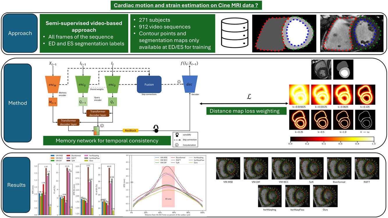
- The paper adapts a video object segmentation architecture, originally built to track objects like people through ordinary video, to track heart wall motion across an entire cardiac MRI cycle.
- Only two frames per cardiac cycle, the most relaxed and most contracted phases, typically have expert segmentation labels. The method makes productive use of every other, unlabeled frame in between.
- A distance map built from the labeled frame weights the training loss so the network prioritizes accuracy near the heart muscle’s actual boundaries rather than treating every pixel equally.
- Tracking error, measured as end point error, dropped to 1.02 millimeters without distance maps and 0.95 millimeters with them, beating every one of eight competing registration and optical flow methods tested, including RAFT at 1.19 millimeters.
- The semi-supervised version, using only two labeled frames per cycle, came within a hair of a fully supervised version that had labels for every single frame, suggesting the expensive part of building a dataset like this may not be necessary.
- Global strain correlations with reference measurements reached 0.83 to 0.91 across the heart’s chambers and deformation types, though regional, segment level strain was noticeably less reliable, a limitation the authors are explicit about.
Why measuring a heartbeat is harder than it sounds
Myocardial strain is a measure of how much the heart muscle itself deforms as it contracts and relaxes, not just how much blood volume moves, and that distinction matters clinically. Strain has become a genuinely useful diagnostic signal for heart failure, myocardial infarction, and various cardiomyopathies, and it also gives clinicians a way to track how a patient is responding to treatment or surgery over time. Cardiac MRI, particularly the cine sequences that capture the heart moving through a full cardiac cycle, is well suited to measuring it, offering high resolution, good signal to noise, and views in multiple planes.
The traditional gold standard, tagged MRI, works by overlaying a magnetic grid pattern onto the heart muscle and watching how that grid deforms as tissue contracts, which gives a very direct readout of motion. But the tags fade as the heart moves through the cycle, and tagging sequences are not part of routine clinical scanning at most centers. That has pushed the field toward feature tracking on ordinary, untagged cine MRI instead, following landmarks near the heart muscle’s inner and outer boundaries across every frame and computing strain from how the distance between neighboring landmarks changes.
The real obstacle to doing this well with deep learning is not the imaging, it is the labels. Precisely outlining the heart muscle’s boundary on every single frame of a cardiac video requires a trained clinical expert and takes real time, so in practice only two frames per cycle typically get annotated, the end diastolic phase, when the heart is most relaxed, and the end systolic phase, when it is most contracted. Everything in between is usually left unlabeled. Prior methods have handled this in one of two unsatisfying ways. Either they train only on the labeled pairs, which throws away most of the video and gives the network very little data to learn from, or they train on every frame without any segmentation supervision at all, which tends to produce less accurate motion right where it matters most, near the muscle’s actual boundary.
The other problem prior methods didn’t fully solve
There is a second, subtler issue the authors identify. Because only the end diastolic and end systolic frames are typically labeled, most training setups only ever show the network motion between those two extremes, which happens to be the largest and hardest motion to estimate in the entire cycle. Most existing strain estimation methods also only ever look at pairs of frames or volumes at training time, which means the network never gets to see the history of how a deformation built up gradually across the cycle, only isolated snapshots. That can produce jumpy, temporally incoherent motion estimates, since the network has no memory of what it predicted a moment ago to keep its next prediction consistent.
Borrowing an architecture built for tracking people in video
The core idea here is a genuine cross pollination between two normally separate fields. In ordinary computer vision, video object segmentation asks a network to track a specific object, a person, a car, an animal, across every frame of a video after being told what that object looks like in just the first frame. A well known architecture for this, Space-Time Memory networks, does this by keeping a running memory of what the object has looked like so far and comparing each new frame against that memory to figure out where the object has moved. The authors realized this is structurally almost identical to the cardiac motion problem. The heart muscle in the end diastolic frame is the object being tracked, and every subsequent frame in the cycle is asking where that same muscle has moved to.
Their network has two parallel encoders working at each step. A query encoder extracts features from whatever frame is currently being processed. A separate memory encoder compresses the accumulated motion information between the very first frame and the most recently processed frame into a compact representation. Unlike the original video segmentation architecture, which keeps a growing bank of memories from every past frame, this network deliberately keeps only the single most recent memory, a simplification the authors found made no measurable difference to accuracy in their own experiments while keeping memory and compute costs down considerably.
At the network’s lowest resolution, the current frame’s features attend to both the previous frame’s features and the compressed memory using standard transformer cross-attention layers, essentially letting the network ask, given what I saw last and what I remember accumulating, where does the muscle boundary sit now. A convolutional GRU layer then folds that attended information forward in time, giving the network an explicit, learned form of short term memory that helps keep successive frame predictions temporally consistent rather than jittery. A U-Net style decoder, modified with residual connections and a more involved skip connection scheme that also pulls in query and memory features at every resolution rather than just the encoder’s own features, then produces the final motion estimate.
Building up motion one small step at a time
Rather than trying to estimate the full, large displacement between the first and current frame directly, which the authors argue is a much harder learning problem, the network works iteratively. At each new frame, it estimates only the small residual motion since the previous frame, then adds that residual on top of the accumulated motion estimate carried forward from all prior steps.
Here F subscript 1,t is the total estimated motion from the first frame to frame t, and the network f only ever has to predict the small increment added at each step. This is a genuinely sensible design choice, since asking a network to directly estimate a large, complex deformation in one shot is a much harder regression target than asking it to estimate a small nudge repeatedly, and the accumulated error from many small nudges, it turns out from the paper’s own ablation, is still meaningfully lower than trying to jump straight to the answer.
The input fed to the memory encoder at each step, denoted X, is itself informative. It concatenates the original first frame, the previous frame, the accumulated motion estimate so far, and an error map showing where the currently warped image disagrees with the true first frame.
That error term matters more than it might first appear. It gives the network a direct, explicit signal about where its own past predictions have gone wrong, which the ablation study shows genuinely helps, particularly for the hardest, largest motions between the most relaxed and most contracted phases of the cycle.
Making the sparse labels count for more
The genuinely novel contribution sits in how the two labeled frames per cycle get used. Rather than only computing a segmentation loss at those two frames and ignoring the rest, the authors generate a distance map from the end diastolic segmentation label, a smooth field where pixels near the heart muscle’s actual anatomical boundaries, the right ventricle, the left ventricular cavity, and the left ventricular myocardium’s inner and outer walls, get high values, and pixels far from those boundaries get low values.
Here x is each pixel’s distance to the nearest anatomical contour, and the formula is the derivative of a sigmoid function, rescaled so its maximum value is exactly one right at the boundary itself, tapering smoothly away from it. This distance map then multiplies into every pixel’s contribution to the similarity and smoothness loss terms used across every single frame of training, not just the two labeled ones, which means the unlabeled frames in between still benefit from knowing roughly where the important anatomical structure sits, borrowed entirely from the one frame that does have a label. The authors also experiment with raising this map to a power k, which sharpens the contrast between high and low weighted regions, and found that pushing k toward its most extreme, effectively a binary mask of the boundary region, gave the best validation accuracy.
A genuine segmentation loss, comparing the reference end diastolic label against the label warped forward using the predicted motion, is applied but only at the end systolic frame, the second point in the cycle that actually has ground truth to check against. That is the semi-supervised part of the recipe. Two labeled frames provide direct segmentation supervision, and the distance map derived from just one of those two labels quietly improves training on every other frame in between.
How well the method actually tracks a beating heart
The dataset behind these results is a genuinely solid one for this kind of study, 271 patients scanned at 1.5 Tesla across two different MRI manufacturers, split into three clinically distinct groups, 96 healthy controls, 114 patients with a genetic cholesterol disorder, and 61 patients with aortic valve stenosis causing left ventricular thickening and stiffness, giving 912 total cardiac sequences with between 20 and 80 frames each.
Tracking accuracy is measured as end point error, the distance in millimeters between where the model predicts a heart muscle boundary point has moved and where an independently validated tracking method, itself checked against manual review, says it actually moved.
| Method | End point error (mm) | F1-all, error over 3mm (%) |
|---|---|---|
| VoxelMorph, MSE loss | 1.21 | 6.12 |
| VoxelMorph, NCC loss | 1.17 | 5.80 |
| VoxelMorph, diffeomorphic | 1.21 | 6.00 |
| Bioinformed (biomechanics-informed regularization) | 1.34 | 6.46 |
| RAFT | 1.19 | 4.95 |
| SyN, classical registration | 1.57 | 13.13 |
| Iterative warping baselines (image and flow) | 1.46 to 1.50 | 11.93 to 12.26 |
| Proposed method (no distance map, fair comparison) | 1.02 | 3.48 |
Every difference between the proposed method and RAFT, its closest competitor overall, was statistically significant across every anatomical structure tracked, right ventricle, left ventricular epicardium, and left ventricular endocardium. It is worth flagging that this comparison table deliberately turns the distance map weighting off for the proposed method, so the comparison isolates the architecture itself rather than mixing in the extra benefit from the loss weighting trick. With distance maps switched back on, the method’s error dropped further still, to 0.95 millimeters, edging close to the 0.91 millimeters achieved by a fully supervised version of the same architecture trained with segmentation labels on every single frame rather than just two per cycle.
The gap widens exactly where it matters most
Perhaps the most clinically relevant result in the paper is how the performance gap between methods changes depending on how far a given frame sits from the end diastolic reference frame. As the amount of accumulated motion increases moving toward the end systolic phase, roughly the midpoint of the cycle, competing methods degrade noticeably, with several baseline approaches showing end point error climbing above 2.5 millimeters right around peak systole. The proposed method’s error also rises in that same region but by a much smaller margin, staying under 1.5 millimeters even at its worst point. That widening gap under harder, larger motion is exactly the scenario the iterative aggregation and memory design were built to handle, and the fact that it shows up cleanly in the data is a reasonably strong validation of that specific design choice.
How the strain numbers themselves held up
Tracking accuracy is a means to an end here, the actual clinical output is strain, and the paper reports separate correlation results for that. For the semi-supervised method with distance maps, correlation with reference peak systolic strain values reached 0.83 for left ventricular global radial strain, 0.90 for left ventricular global circumferential strain, and 0.91 for right ventricular global circumferential strain, with correlations on the timing of when that peak occurs running even higher, generally above 0.94. Notably, the fully supervised version, using every frame’s labels rather than just two, only improved on these numbers marginally, again reinforcing that the semi-supervised recipe is capturing most of the achievable accuracy.
Regional, segment level strain, breaking the myocardium down into six anatomical wall segments rather than reporting one global number for the whole ventricle, was noticeably less reliable, with correlations generally in the 0.60 to 0.81 range depending on the specific segment and strain type. The authors are direct about this limitation, stating plainly that regional strain results are not yet close enough to reference measurements to be used reliably in a clinical setting, while global strain, they argue, is ready for that kind of use given how strongly it correlated and how much more reproducible global strain measurements have been shown to be in prior clinical literature.
What the ablation study reveals about the design choices
Removing the convGRU temporal memory layer caused only a small drop in accuracy, a modestly disappointing result for a component that sounds architecturally central, though the authors note it still contributes meaningfully to keeping predictions temporally smooth even if the raw accuracy cost of removing it is small. Removing the iterative aggregation process entirely, having the network try to predict the full motion from the first frame directly in one step rather than accumulating small residuals, caused a considerably larger drop, especially for the hardest end diastolic to end systolic motion, which is good evidence that the incremental, memory driven design is doing real work rather than adding complexity for its own sake.
The number of frames sampled during training also mattered up to a point. Training with only two frames per sequence, effectively collapsing back to a standard pairwise registration setup, produced dramatically worse results, an end point error above 2 millimeters. Accuracy improved steadily as more frames were included, but the gains largely leveled off around seven or eight frames, with the paper’s default of twelve frames offering little additional benefit beyond that plateau. That is a useful practical data point for anyone trying to replicate this approach with tighter GPU memory constraints, since seven or eight frames appears to capture most of the achievable benefit at a meaningfully lower training cost than twelve.
Clinical translation gap
It is worth being precise about the distance between this result and something a hospital could deploy tomorrow. The entire dataset comes from a single research collaboration, albeit collected across different scanner vendors and patient groups, rather than from an independently sourced external validation cohort at a different institution, the kind of test that speaks most directly to whether a method generalizes beyond the exact conditions it was built and tuned under. The reference values the model is being checked against are themselves not a true independent gold standard like tagged MRI or DENSE, but rather the output of the authors’ own in-house semi-automatic feature tracking software, which, while shown in prior work to be highly reproducible, is still a computational proxy for ground truth rather than ground truth itself. And the paper’s own regional strain results, by the authors’ explicit admission, are not yet accurate enough for segment level clinical decision making, meaning the method’s near clinical readiness claim applies specifically to global, whole chamber strain rather than to the finer grained regional analysis that can matter for localizing specific areas of muscle damage after a heart attack.
Clinical limitations reported or implied in the paper
- All 271 patients came from the same research collaboration and imaging protocol, with no independently sourced external test set from a different center or scanner setup used to check generalization.
- The reference strain and tracking values used to validate the model come from the authors’ own semi-automatic feature tracking software rather than an independent gold standard imaging technique such as tagged MRI or DENSE.
- Regional, segment level strain correlations, generally in the 0.60 to 0.81 range, are explicitly flagged by the authors as not yet reliable enough for clinical use, limiting the near ready claim to global strain measurements only.
- The dataset’s three patient groups, healthy controls, a hereditary cholesterol disorder, and aortic valve stenosis, do not include patients with confirmed myocardial infarction, one of the primary conditions strain imaging is used to help diagnose, so performance on infarcted, scarred myocardium specifically remains untested here.
Where this fits against the rest of the field
The comparison set in this paper is genuinely comprehensive by the standards of the medical image registration literature, spanning three variants of VoxelMorph, a classical non-learning registration algorithm, a recent biomechanics-informed neural approach, the well established RAFT optical flow model, and two intuitive but naive baselines that simply chain together pairwise registrations frame by frame. Beating all eight by a statistically significant margin on the same retrained, apples to apples comparison, rather than citing each method’s own reported numbers from its original paper, is a methodologically sound way to run this kind of benchmark and gives the result more credibility than a table of numbers pulled from different papers with different datasets would.
The architectural borrowing from video object segmentation is, as far as the authors are aware, a genuinely first attempt at combining that specific memory network design with order learning style biomechanical tracking in the cardiac imaging space. That kind of cross pollination, taking an architecture solved for a structurally similar but domain distant problem and re-purposing it, tends to be a productive move in medical imaging generally, and the fact that it produced a clean, statistically significant improvement over methods purpose built for cardiac motion, like the biomechanics-informed model, is a reasonably strong argument that the general recipe, not just the medical domain specific tricks layered on top, is doing meaningful work.
Limitations worth taking seriously
A handful of things beyond the clinical translation gap deserve a skeptical read. The paper’s own regression analysis of performance against pixel size found a moderate positive correlation, meaning error tends to increase with coarser pixel resolution, but the authors themselves caution this finding rests on a small number of data points and appears to be disproportionately driven by just two outlier scans from one manufacturer, which is honest but also means the pixel size finding should not be treated as a settled result. The claim that using segmentation labels on every frame provides little additional benefit over the semi-supervised two frame approach is a genuinely interesting and useful result, but it rests on comparing against a single in-house dataset and a single choice of network architecture, so it is not yet clear how far that finding generalizes to other cardiac motion architectures or other anatomical tracking problems. Finally, while the statistical testing throughout is appropriately rigorous, using the Wilcoxon signed-rank test for paired comparisons and reporting p-values consistently, the practical, clinical significance of a difference measured in fractions of a millimeter is a separate question from statistical significance that the paper does not directly address, and readers should keep that distinction in mind when weighing how much the reported improvements would actually change a clinical reading.
Conclusion
The core achievement here is a genuinely clever repurposing of video object segmentation machinery for a medical tracking problem that shares more structural similarity with mainstream computer vision than it might first appear, combined with a distance map weighting trick that squeezes real additional value out of the two labeled frames every cardiac dataset already has, without requiring the expensive, expert time intensive work of labeling every frame in between. Beating eight established registration and optical flow baselines on a rigorously matched, retrained comparison, and coming within 0.04 millimeters of a fully supervised alternative using a fraction of the labeling effort, is a substantial and well demonstrated result.
The idea most likely to travel beyond cardiac imaging specifically is the general recipe, not the cardiac specific tricks. Any medical video tracking problem with the same sparse annotation pattern, two or a handful of labeled frames surrounded by many unlabeled ones, and where getting the boundary of some anatomical structure right matters more than getting the background right, could plausibly benefit from the same combination of an iterative, memory driven architecture and a distance map derived loss weighting scheme built from whatever sparse labels are available.
The honest remaining gap is the one the authors themselves are candid about. Global strain looks close to something clinically usable. Regional strain, which is often what matters most for localizing damage after an infarction specifically, is not there yet, and the paper’s own suggested next steps, incorporating anatomical landmarks, biomechanical priors around tissue incompressibility, and richer forms of intermediate frame supervision, read as a reasonable and specific roadmap rather than a vague gesture at future work. None of that undercuts what has already been demonstrated. It just means the realistic next step is closing that regional strain gap and validating on an external, independently sourced cohort, not a jump to bedside deployment.
The authors’ own conclusion points toward extending the approach to all four heart chambers and both short and long axis MRI views, and toward using biophysical heart models to synthesize additional training data as a way to strengthen validation further. Both are sensible, achievable extensions of a method that has already cleared a meaningfully high bar against the existing state of the art in cardiac motion tracking.
Frequently asked questions
What is myocardial strain and why does it matter clinically
Myocardial strain measures how much the heart muscle itself deforms as it contracts and relaxes through a cardiac cycle, which gives clinicians a more direct readout of pumping efficiency than blood volume measurements alone, and it is used to help diagnose heart failure, myocardial infarction, and various cardiomyopathies.
Why did the researchers borrow an architecture from video object segmentation
Tracking a heart muscle boundary across the frames of a cardiac MRI video is structurally very similar to tracking a specific object, like a person or a car, across the frames of ordinary video, since both problems involve locating the same structure in every subsequent frame after being shown where it starts in the first one.
How does the model make use of frames that were never manually labeled
A distance map computed from the one labeled reference frame is used to weight the training loss on every frame in the sequence, giving the network a sense of where the important anatomical boundaries roughly sit even on frames that have no direct segmentation label of their own.
Is labeling every frame of a cardiac MRI video still necessary for this to work well
Not really, according to this paper. The semi-supervised version, trained with labels on only two frames per cardiac cycle, came within 0.04 millimeters of end point error compared to a fully supervised version trained with labels on every single frame.
Does this method work equally well for whole heart strain and for specific wall segments
No. Correlations for global, whole chamber strain reached 0.83 to 0.91 against reference measurements, but correlations for regional, segment level strain were noticeably lower, generally in the 0.60 to 0.81 range, and the authors explicitly state regional strain is not yet accurate enough for reliable clinical use.
Has this method been tested on patients with confirmed heart attacks
The dataset used includes healthy controls, patients with a hereditary cholesterol disorder, and patients with aortic valve stenosis, but not patients with confirmed myocardial infarction specifically, so performance on scarred, infarcted heart tissue has not yet been directly demonstrated in this paper.
Reproducible implementation sketch
The block below is an independent implementation of the core architectural ideas in the paper, a query and memory dual encoder with transformer cross-attention and a convGRU, iterative residual motion aggregation, and distance map weighted losses, written in PyTorch. It is a starting point for experimentation, not a copy of the authors’ original code, which was not released publicly at the time of writing.
# cardiac_memory_flow.py
# Independent reproduction of the core ideas in Portal et al., Computers in
# Biology and Medicine 2025, semi-supervised cardiac motion via a memory network

import torch
import torch.nn as nn
import torch.nn.functional as F


class ConvEncoder(nn.Module):
    """Shared style encoder, used for both the query and memory paths, that
    downsamples an input tensor to 1/8 resolution feature maps."""

    def __init__(self, in_channels, base_dim=64, feat_dim=256):
        super().__init__()
        self.net = nn.Sequential(
            nn.Conv2d(in_channels, base_dim, 7, stride=2, padding=3),
            nn.GroupNorm(8, base_dim), nn.ReLU(inplace=True),
            nn.Conv2d(base_dim, base_dim * 2, 3, stride=2, padding=1),
            nn.GroupNorm(8, base_dim * 2), nn.ReLU(inplace=True),
            nn.Conv2d(base_dim * 2, feat_dim, 3, stride=2, padding=1),
            nn.GroupNorm(8, feat_dim), nn.ReLU(inplace=True),
        )

    def forward(self, x):
        return self.net(x)  # (B, feat_dim, H/8, W/8)


class CrossAttentionBlock(nn.Module):
    """Standard transformer cross attention, Query attends to Key/Value,
    used both for Q_t attending to Q_t-1 and Q_t attending to (Q_1, M_t-1)."""

    def __init__(self, dim, num_heads=8):
        super().__init__()
        self.attn = nn.MultiheadAttention(dim, num_heads, batch_first=True)
        self.norm = nn.LayerNorm(dim)

    def forward(self, query, key, value):
        # flatten spatial dims to a sequence for attention, then reshape back
        B, C, H, W = query.shape
        q = query.flatten(2).transpose(1, 2)  # (B, H*W, C)
        k = key.flatten(2).transpose(1, 2)
        v = value.flatten(2).transpose(1, 2)
        out, _ = self.attn(q, k, v)
        out = self.norm(out + q)
        return out.transpose(1, 2).reshape(B, C, H, W)


class ConvGRUCell(nn.Module):
    """Convolutional GRU that folds attended features forward across the
    iterative aggregation steps, giving the network short term memory."""

    def __init__(self, dim):
        super().__init__()
        self.update_gate = nn.Conv2d(dim * 2, dim, 3, padding=1)
        self.reset_gate = nn.Conv2d(dim * 2, dim, 3, padding=1)
        self.candidate = nn.Conv2d(dim * 2, dim, 3, padding=1)

    def forward(self, x, hidden):
        combined = torch.cat([x, hidden], dim=1)
        z = torch.sigmoid(self.update_gate(combined))
        r = torch.sigmoid(self.reset_gate(combined))
        candidate_input = torch.cat([x, r * hidden], dim=1)
        candidate = torch.tanh(self.candidate(candidate_input))
        return (1 - z) * hidden + z * candidate


class FlowDecoder(nn.Module):
    """Upsamples fused query/memory features back to full resolution and
    predicts a 2 channel residual flow (dx, dy)."""

    def __init__(self, feat_dim=256):
        super().__init__()
        self.up1 = nn.ConvTranspose2d(feat_dim, 128, 4, stride=2, padding=1)
        self.up2 = nn.ConvTranspose2d(128, 64, 4, stride=2, padding=1)
        self.up3 = nn.ConvTranspose2d(64, 32, 4, stride=2, padding=1)
        self.flow_head = nn.Conv2d(32, 2, 3, padding=1)

    def forward(self, x):
        x = F.relu(self.up1(x))
        x = F.relu(self.up2(x))
        x = F.relu(self.up3(x))
        return self.flow_head(x)  # (B, 2, H, W) residual flow


class CardiacMemoryFlowNet(nn.Module):
    """Iteratively aggregates motion from the first (ED) frame to every
    subsequent frame using a query/memory dual encoder with cross attention
    and a convGRU, matching the paper's core design."""

    def __init__(self, feat_dim=256):
        super().__init__()
        self.query_encoder = ConvEncoder(in_channels=1, feat_dim=feat_dim)
        self.memory_encoder = ConvEncoder(in_channels=5, feat_dim=feat_dim)  # [I1, It-1, Fx, Fy, E]
        self.attn_prev_query = CrossAttentionBlock(feat_dim)
        self.attn_memory = CrossAttentionBlock(feat_dim)
        self.fuse = nn.Conv2d(feat_dim * 2, feat_dim, 3, padding=1)
        self.gru = ConvGRUCell(feat_dim)
        self.decoder = FlowDecoder(feat_dim)

    def warp(self, image, flow):
        """Backward warps `image` using `flow`, matching Eq. 1-2 in the paper,
        via a differentiable grid sample (the spatial transformer building block)."""
        B, C, H, W = image.shape
        yy, xx = torch.meshgrid(
            torch.linspace(-1, 1, H, device=image.device),
            torch.linspace(-1, 1, W, device=image.device),
            indexing="ij",
        )
        base_grid = torch.stack([xx, yy], dim=-1).unsqueeze(0).expand(B, -1, -1, -1)
        flow_norm = torch.stack(
            [flow[:, 0] / (W / 2), flow[:, 1] / (H / 2)], dim=-1
        )
        sample_grid = base_grid + flow_norm
        return F.grid_sample(image, sample_grid, align_corners=True)

    def forward(self, sequence):
        """sequence: (B, T, 1, H, W), a full cardiac cycle sub-sequence, with
        frame 0 as the ED reference frame. Returns the accumulated motion
        flow from frame 0 to every other frame, (B, T-1, 2, H, W)."""
        B, T, _, H, W = sequence.shape
        device = sequence.device

        I1 = sequence[:, 0]
        F1_t = torch.zeros(B, 2, H, W, device=device)  # F1,1 = 0
        hidden = torch.zeros(B, 256, H // 8, W // 8, device=device)

        Q1 = self.query_encoder(I1)
        Q_prev = Q1
        all_flows = []

        for t in range(1, T):
            It = sequence[:, t]
            I_prev = sequence[:, t - 1]

            # build X_{t-1} = [I1, I_{t-1}, F1_{t-1}, E_{t-1,1}]
            R_prev = self.warp(I_prev, F1_t)
            E_prev = R_prev - I1
            memory_input = torch.cat([I1, I_prev, F1_t, E_prev], dim=1)
            M_prev = self.memory_encoder(memory_input)

            Qt = self.query_encoder(It)
            B1 = self.attn_prev_query(Qt, Q_prev, Q_prev)
            B2 = self.attn_memory(Qt, Q1, M_prev)
            fused = F.relu(self.fuse(torch.cat([B1, B2], dim=1)))

            hidden = self.gru(fused, hidden)
            residual_flow = self.decoder(hidden)  # small residual, low res upsampled to full res

            F1_t = F1_t + residual_flow  # Eq. 6, iterative aggregation
            all_flows.append(F1_t)
            Q_prev = Qt

        return torch.stack(all_flows, dim=1)  # (B, T-1, 2, H, W)


def distance_map_weighted_ncc_loss(I1, warped, distance_map):
    """Local normalized cross correlation similarity loss weighted by the
    ED distance map, matching Eq. 12. A simplified windowed NCC is used here."""
    mean1 = F.avg_pool2d(I1, 9, stride=1, padding=4)
    mean2 = F.avg_pool2d(warped, 9, stride=1, padding=4)
    var1 = F.avg_pool2d(I1 * I1, 9, stride=1, padding=4) - mean1 ** 2
    var2 = F.avg_pool2d(warped * warped, 9, stride=1, padding=4) - mean2 ** 2
    cov = F.avg_pool2d(I1 * warped, 9, stride=1, padding=4) - mean1 * mean2
    ncc = cov / (torch.sqrt(var1 * var2) + 1e-5)
    return (distance_map * (1 - ncc)).mean()


def distance_map_weighted_smoothness_loss(flow, distance_map):
    """Penalizes spatial gradients of the flow, weighted by the distance
    map, matching Eq. 13."""
    dx = flow[:, :, :, 1:] - flow[:, :, :, :-1]
    dy = flow[:, :, 1:, :] - flow[:, :, :-1, :]
    dx_sq = (dx ** 2).sum(dim=1, keepdim=True)
    dy_sq = (dy ** 2).sum(dim=1, keepdim=True)
    loss_x = (distance_map[:, :, :, 1:] * dx_sq).mean()
    loss_y = (distance_map[:, :, 1:, :] * dy_sq).mean()
    return loss_x + loss_y


def compute_distance_map(segmentation_mask, k=4.0):
    """Converts a binary contour mask into the smooth distance map used to
    weight the losses, matching Eq. 11, using a simple Euclidean distance
    transform substitute suitable for a differentiable pipeline sketch."""
    import scipy.ndimage as ndi
    mask_np = segmentation_mask.detach().cpu().numpy()
    dist = ndi.distance_transform_edt(1 - mask_np)
    delta = 4 * torch.exp(-torch.tensor(dist)) / (1 + torch.exp(-torch.tensor(dist))) ** 2
    return (delta ** k).float()


def smoke_test():
    """Runs one forward pass through the network on random dummy data to
    confirm shapes line up, and checks the distance map weighted losses."""
    device = torch.device("cuda" if torch.cuda.is_available() else "cpu")
    model = CardiacMemoryFlowNet().to(device)

    B, T, H, W = 1, 6, 128, 128
    dummy_sequence = torch.randn(B, T, 1, H, W, device=device)

    flows = model(dummy_sequence)
    assert flows.shape == (B, T - 1, 2, H, W)
    print(f"forward pass ok, output flow shape {tuple(flows.shape)}")

    I1 = dummy_sequence[:, 0]
    warped = model.warp(dummy_sequence[:, -1], flows[:, -1])
    dummy_distance_map = torch.rand(B, 1, H, W, device=device)

    sim_loss = distance_map_weighted_ncc_loss(I1, warped, dummy_distance_map)
    smooth_loss = distance_map_weighted_smoothness_loss(flows[:, -1], dummy_distance_map)
    print(f"similarity loss {sim_loss.item():.4f}, smoothness loss {smooth_loss.item():.4f}")


if __name__ == "__main__":
    smoke_test()
This analysis is based on the published paper and an independent evaluation of its claims.
Can you be more specific about the content of your article? After reading it, I still have some doubts. Hope you can help me. https://accounts.binance.info/register-person?ref=QCGZMHR6
Thanks for sharing. I read many of your blog posts, cool, your blog is very good. https://www.binance.info/register?ref=QCGZMHR6
Thank you for your sharing. I am worried that I lack creative ideas. It is your article that makes me full of hope. Thank you. But, I have a question, can you help me?
Your point of view caught my eye and was very interesting. Thanks. I have a question for you. https://www.binance.com/register?ref=IHJUI7TF