
- Monte Carlo rendering
- Signed distance functions
- Volumetric emitters
- Next event estimation
- Importance sampling
- Sphere tracing
- PyTorch
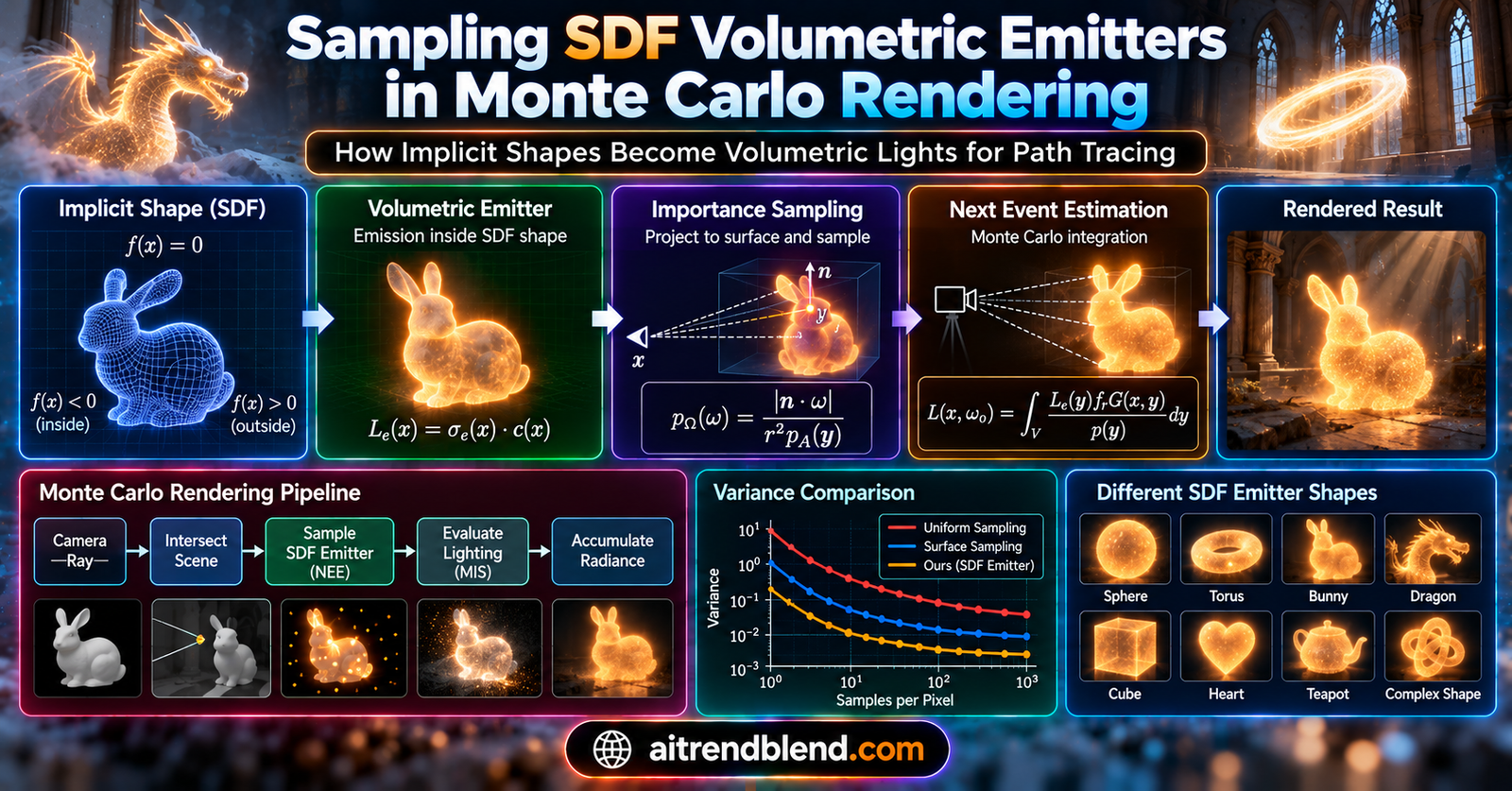
A lighting artist on an animated film wants a lamp that glows from the inside, shaped like a knotted fractal that a shader programmer wrote in forty lines of code. The renderer can draw that shape easily. It cannot light the room with it. To use the lamp as a light source, the artist has to convert the fractal into a dense triangle mesh, wait for the renderer to build a sampling structure over hundreds of thousands of tiny emitting triangles, and accept that the glow now lives only on the surface.
A team from the International Digital Economy Academy in Shenzhen, Tsinghua University and Tohoku University decided that workaround was unnecessary. Their paper shows how to sample light directly from the interior of any shape defined by a signed distance function, with no meshing and no precomputed tables. The core trick is one change of variables, and it turns out to hide some quietly elegant probability.
Key points
- The method treats the inside of a signed distance function as a uniformly glowing volume, picks random points inside it, and turns each point into a direction as seen from the surface being shaded.
- That projection induces a directional probability density with a closed form, one third of the sum of cubed segment lengths along the ray divided by the volume.
- For distant emitters this density becomes proportional to the true radiance, which is the ideal importance sampling target. Near the emitter it overweights deep paths.
- Our analysis shows the estimator is the Rao Blackwell improvement of simply treating each sampled point as a point light, so it can never be noisier than that obvious baseline.
- In the paper’s direct lighting tests, error fell by factors between about 1.3 and 6 against the strongest competing light sampler at equal samples per pixel, with under 30 percent extra render time for the composite shapes.
- Robust sphere tracing is the practical backbone, and our reproduction shows that overestimating distance fields need a Lipschitz correction outside the volume as well as the paper’s clamp inside it.
Why Volumetric Lights Are Awkward in a Path Tracer
A path tracer computes the colour of a pixel by estimating an integral over all the light arriving at a surface point. The most important technique for doing this efficiently is next event estimation. At every bounce, instead of waiting for a random ray to stumble onto a light, the renderer deliberately samples a direction toward a light source and asks how much energy arrives from there. How well that sampling matches the true distribution of incoming light decides how noisy the image will be.
For simple lights this problem was solved decades ago. James Arvo showed how to sample spherical triangles uniformly by solid angle in 1995. Carlos Ureña, Marcos Fajardo and Alan King did the same for rectangles in 2013, and Manuel Gamito for disks and cylinders in 2016. Sampling uniformly over the solid angle a flat diffuse light subtends is nearly ideal, because the geometry terms cancel and every sample carries almost the same weight.
Volumetric light sources are messier. Fire, glowing gas and luminous fog are usually stored as voxel grids, and sampling them means integrating emission along rays through the grid, as in the work of Ryusuke Villemin and Christophe Hery and of Florian Simon and colleagues. Grids are memory hungry and blur fine structure. Meanwhile, signed distance functions have become the language of procedural modelling, used everywhere from demoscene shaders to neural surface reconstruction, yet almost nobody uses them as lights. The reason is not that volumetric emitters are bad. As the authors put it, the gap comes from the difficulty of sampling and integrating them.
Jiawei Huang, Shaokun Zheng, Kun Xu, Yoshifumi Kitamura and Jiaping Wang close that gap in their paper in Computational Visual Media, volume 12, 2026. The site’s Math Applications hub collects other papers where, as here, a little well chosen mathematics does most of the work, such as our analysis of how CAST speeds up approximate Cholesky with random spanning trees.
The Emission Model
Start with a signed distance function \( \varphi : \mathbb{R}^3 \to \mathbb{R} \), negative inside the shape and positive outside. The emitting region is \( \Omega = \{x : \varphi(x) \le 0\} \), and its indicator \( v(x) \) is 1 inside and 0 outside. The total volume is \( V = \int v(x)\,dx \).
A volumetric emitter radiates from every interior point. If \( \rho(x) \) is the emission per unit length, the radiance arriving at a shading point \( x_0 \) from direction \( \omega \) is the line integral of emission along that ray.
The second form splits the ray into the intervals \( [r_i^-, r_i^+] \) where it passes through the interior. A ray through a torus can cross it twice, a ray through a fractal many times. For uniform emission the authors set \( \rho = 1/V \) so the emitter has unit total power, and the integral becomes a sum of chord lengths.
For spatially varying emission they draw one uniform point \( r^{*} \) inside each segment and use \( \sum_i (r_i^+ – r_i^-)\,\rho(x_0 + r^{*}\omega) \), an unbiased one sample estimate of each segment’s integral. Brightness in this model depends on how much glowing material the ray passes through, which is exactly how a real luminous gas behaves.
From a Random Point to a Random Direction
The renderer needs directions, but for an implicit shape it is much easier to produce points. Rejection sampling works for any shape. Draw points uniformly in a bounding box and keep the ones where \( \varphi \le 0 \). For simple primitives there are direct formulas. A uniform point in a sphere of radius R has radius \( R u^{1/3} \) and a uniform direction.
The key idea of the paper is to take such a point \( x \), uniform over the interior with density \( 1/V \), and project it onto the unit sphere around the shading point.
This gives a random direction, but a random direction is only useful for importance sampling if you can also evaluate its probability density. The density follows from a change to spherical coordinates centred at the shading point, \( x = x_0 + r\omega \), for which the volume element is \( dx = r^2\,dr\,d\omega \). The joint density of distance and direction is therefore \( v(x_0 + r\omega)\,r^2 / V \), and integrating out the distance gives the directional density.
That is the central formula. The same ray query that computes the radiance in Equation 2 also computes the density, because both only need the entry and exit distances. No mesh, no voxel grid and no table over directions is required.
Our reproduction checks that this density really integrates to one over the sphere of directions, from a shading point outside a torus and from one inside its tube. The Monte Carlo estimates came out at 1.006 and 0.998, each within about one standard error of 1.
Why the r squared factor matters
The ideal density for next event estimation with a uniform emitter is proportional to the radiance itself, \( p^{*}(\omega) \propto \sum_i (r_i^+ – r_i^-) \), because then every sample carries the same weight. The projection density is proportional to a sum of cubes instead. For a single segment the cube factors neatly.
When the emitter is far away compared with its thickness, both distances are close to some D, the bracket is close to \( 3D^2 \), and the projection density is proportional to the chord length. In that regime the method samples almost exactly in proportion to the light. Near the emitter the bracket favours segments that are further away, which the authors describe as a safe heuristic that overweights the core of the emitter.
It helps to write down the actual Monte Carlo weight, which the paper does not state explicitly. With uniform emission of total power \( I \), divide Equation 2 by Equation 4 for a single segment. The volume cancels.
This is a smoothed inverse square law. It depends only on how far away the segment is, not on how thick it is. So the variance of the estimator comes almost entirely from the spread of distances to different parts of the emitter. That explains the far field behaviour directly. In our torus experiment, the coefficient of variation of this weight across samples was 0.013 with the shading point 1.5 units above the centre, 0.004 at 3 units and effectively zero at 10.
It also exposes the weak spot. If the shading point sits inside the emitter, \( r^- = 0 \) and the weight becomes \( 3I/(r^+)^2 \). Directions that exit the volume quickly get very large weights. We return to this below.
A Hidden Connection, Rao Blackwell
There is a simpler way to use a uniform interior point, and it is worth comparing against. Treat the sampled point as a tiny point light. For uniform emission, the irradiance at a surface with normal \( n \) is \( E = \int L_e(\omega)\,\max(0, n\cdot\omega)\,d\omega \), and the same change of variables turns it into a volume integral, \( E = \frac{I}{V}\int_{\Omega} \frac{\max(0, n\cdot\omega_x)}{\Vert x – x_0\rVert^{2}}\,dx \). Sampling \( x \) uniformly gives the point light estimator \( I\max(0, n\cdot\omega)/r^2 \).
Now ask what this estimator averages to if you fix the direction and let only the distance vary. Given \( \omega \), Equation 4 says the distance has density proportional to \( r^2 \) on the ray’s interior segments. The conditional expectation is therefore easy to compute.
The right hand side is exactly the paper’s estimator. In statistical language, the projection estimator is the Rao Blackwell improvement of the point light estimator, obtained by integrating out the distance along the ray analytically. By the law of total variance it can never be noisier. The sphere traced line integral is not just a convenience for evaluating the PDF. It is what buys the variance reduction over the obvious alternative. Readers of our knowledge distillation mathematics explainer will recognise the same law of total variance argument, there used to explain why soft labels help.
The difference can be large. With the shading point outside the torus, our reproduction measured a per sample variance of 0.0058 for the point light estimator and 0.0037 for the projection estimator, a 1.6 times improvement. With the shading point inside the tube, the point light estimator’s \( 1/r^2 \) term has infinite variance, because \( \int (r^{-2})^{2} r^{2}\,dr \) diverges at zero. Its sample variance came out at about 35 and its mean was visibly wrong at 0.656 against a true value near 0.709. The projection estimator’s weight in Equation 6 is bounded by the distance to the nearest exit, so it stayed finite.
Sampling a point inside the emitter and projecting it to a direction is the natural idea. What makes it good is evaluating the full line integral along that direction. That integral turns a heavy tailed point light estimator into its Rao Blackwellized version, which is never worse and removes the infinite variance when the shading point is inside the light.
Finding Every Entry and Exit
Both Equation 2 and Equation 4 need every interval where the ray is inside the shape. For spheres the intervals come from a quadratic, and for a torus from a quartic. For a general SDF, including Boolean combinations and procedural fractals, the authors use sphere tracing, introduced by John Hart in 1996. Outside the shape, the value \( \varphi(x) \) is a safe step, because no surface can be closer than that in any direction.
Inside, the paper adopts what it calls a directional safe step.
Once a step crosses the surface, a few rounds of bisection locate the crossing precisely. The authors recommend setting \( \delta_{\max} \) to the thinnest feature worth resolving, or to the bounding box diagonal divided by a factor between 20 and 100 when that is unknown, and used a single value of 0.05 in normalized emitter coordinates for every scene in the paper.
The justification deserves a careful reading. The paper argues that stepping by \( |\varphi| \) inside can overshoot the next crossing, particularly at grazing incidence. For a true distance field this cannot happen. A ball of radius \( |\varphi(x)| \) around \( x \) contains no surface point, so a step of that length in any direction stays inside. The paper’s own next sentence identifies the real issue. Constructive solid geometry with smooth blends, domain deformations and voxel reconstructed fields often overestimate the distance, and then the step is no longer safe. The clamp is insurance against fields that are not true distances.
Our reproduction tests this directly with a thin slab followed by two thick slabs separated by a narrow gap. With the exact field, plain sphere tracing found every segment on every ray. We then multiplied the field by 3, which is what a non uniform scale does if the correction factor discussed in the next section is forgotten.
| Distance field and stepping rule | Rays with every segment found | Mean error in interior length |
|---|---|---|
| Exact field, plain sphere tracing | 100% | 0.00% |
| Field times 3, plain sphere tracing | 0% | 12.6% |
| Field times 3, clamped interior step only | 0% | 10.5% |
| Field times 3, clamped interior step and outside step divided by 3 | 100% | 0.00% |
4,000 slightly oblique rays per row, reference from very fine marching. Computed by aitrendblend with the code below.
The clamped interior step alone did not rescue the overestimating field, because the outside step overshot the thin slab entirely before the ray ever got inside. The paper states that the standard outside step remains valid. That holds for fields that are true distance bounds outside, which covers the common cases, but for any field whose Lipschitz constant exceeds one the outside step needs the same care. Dividing it by a Lipschitz bound fixed everything.
We found one more practical wrinkle. A ray that skims the inner surface without crossing it takes interior steps of size \( -\varphi \) that shrink toward zero, the classic sphere tracing slowdown near grazing incidence. In our first run a single such ray stalled for thousands of iterations and was silently dropped. A small minimum step, with bisection catching any crossing inside it, removed the problem.
Transforms, Intensity and the Volume Estimate
Artists expect to move, rotate and scale a light. For a world transform \( x’ = RSx + t \) with diagonal scale \( S \), the authors evaluate the transformed field conservatively.
Multiplying by the smallest scale factor keeps the field from overestimating distances after a non uniform stretch. It is precisely the correction whose absence broke the slab test above. Sampling happens in the emitter’s local space, and the directional density picks up a Jacobian factor, \( p'(\omega’) = p(\omega’)/|\det S| \).
One implementation detail is worth making explicit. That formula is exact when the local ray keeps the world distance parameter, meaning the local direction \( S^{-1}R^{-1}\omega \) is not renormalized. If an implementation renormalizes the local direction, an extra factor of \( \Vert S^{-1}R^{-1}\omega\rVert^{-3} \) appears. Our reproduction compared both against a density computed directly in world space for a stretched and rotated ellipsoid. The unnormalized version matched to about \( 10^{-12} \). The renormalized version without the extra factor was off by up to 100 percent, and adding the factor restored agreement.
For shapes without a closed form volume, \( V \) is estimated by Monte Carlo as the bounding box volume times the fraction of random box points that land inside. This is a binomial proportion, so with fill fraction \( f = V/V_{\text{box}} \) and \( N \) samples the relative standard error is \( \sqrt{(1-f)/(fN)} \). The authors report errors below 1 percent by about \( 2^{18} \) samples and a GPU time under 2 milliseconds for \( 2^{31} \) samples. The same formula explains a limitation discussed later. When the shape fills only a small fraction of its box, both the volume estimate and the rejection sampler waste effort in proportion to \( 1/f \).
The authors argue that an estimated volume only rescales brightness by \( V/\hat{V} \). The algebra is more interesting than that. In next event estimation, \( \hat{V} \) appears in both the emitted radiance and the density, and it cancels exactly as in Equation 6. Rays that hit the emitter by BSDF sampling carry the rescaled radiance with no density to cancel it. In our test, inflating \( \hat{V} \) by 5 percent left the next event estimate unchanged and lowered the BSDF sampled estimate by exactly a factor of 1.05. At the paper’s 0.1 percent accuracy that inconsistency is invisible, but it is the reason the estimate needs to be accurate at all.
Every practical ingredient, the interior step clamp, the conservative transform, the Jacobian and the volume estimate, exists to keep one promise. The density used to weight a sample must be the density that actually produced it. When they are consistent, the estimator stays unbiased no matter how odd the shape is.
What the Experiments Show
The authors implemented the method in a proprietary GPU production renderer and also released an implementation built on LuisaCompute with the paper’s supplementary material. Tests ran on a desktop with an NVIDIA RTX 4070 at 1024 by 1024 resolution. Variance comparisons used direct lighting only, 64 samples per pixel and equal sample counts, with error reported as MAPE and the perceptual FLIP metric from Pontus Andersson and colleagues. Lower is better for both.
| Scene and emitter | BSDF sampling only | Competing light sampling | SDF emitter sampling |
|---|---|---|---|
| Dragon, analytic torus | 0.699 / 0.448 | Surface area, 0.078 / 0.054 | 0.024 / 0.021 |
| Room, analytic shapes | 0.755 / 0.647 | Surface area, 0.155 / 0.094 | 0.122 / 0.077 |
| Kitchen, fractal lamp | 0.945 / 0.761 | Bounding volume, 0.079 / 0.083 | 0.013 / 0.020 |
| Corridor, logo emitter | 0.805 / 0.587 | Bounding volume, 0.239 / 0.179 | 0.047 / 0.045 |
MAPE / FLIP at 64 samples per pixel, as reported in Figures 3 and 7 of Huang et al. (2026). Bounding volume sampling applies the same projection method to a box or sphere enclosing the shape.
On the composite shapes the gains are large. In the Kitchen scene MAPE falls about sixfold against bounding volume sampling and roughly seventyfold against BSDF sampling alone, and the authors report that evaluating the exact SDF added less than 30 percent to render time. The bounding volume baseline is instructive. It uses the very same projection idea, only on a proxy shape, so its gap to the full method isolates the value of sampling the true geometry rather than empty space around it.
On the analytic shapes the picture is more mixed. The Dragon scene improves about threefold over surface sampling. The Room scene improves by about a fifth. Surface sampling ignores the interior, so its advantage shrinks when emitters are thin or seen mostly edge on, and the projection method pays for its near field overweighting.
The authors also tested spatially varying emission. MAPE rose from 0.058 to 0.082 in a Pool scene with colour varying across an extruded logo, and from 0.123 to 0.193 in a Hall scene with intensity falling off from the surface. That is the roughly 50 percent increase the paper reports, and the cause is clear from Equation 4. The density follows only the geometry, so any variation in \( \rho \) becomes variation in the weights.
Two further results show why volumetric emitters are worth having. A bunny emitter stored as a small SIREN network with dozens of weights rendered very similarly to its triangle mesh version at two orders of magnitude less memory. And a glowing sphere rendered as a volume casts a noticeably sharper shadow than the same sphere as a surface light, because rays through its centre pass through more glowing material. That directional variation of brightness cannot be imitated by adjusting the intensity of a surface light.
Our Toy Reproduction
To see the estimators side by side, the code at the end computes irradiance from a torus emitter with major radius 1 and tube radius 0.35, using five strategies with 250,000 samples each, or 60,000 for the non uniform case. Wherever the variance is finite, all five agree on the mean to within about one or two standard errors, which is the unbiasedness check. The variances tell the story.
| Strategy | Shading point above the torus | Shading point inside the tube | Above, non uniform emission |
|---|---|---|---|
| Uniform directions | 0.5597 | 0.7608 | 1.3912 |
| Cosine weighted directions | 0.1273 | 0.0712 | 0.3365 |
| Point in volume, inverse square | 0.0058 | about 35, unstable | 0.0580 |
| Projection NEE, the paper’s method | 0.0037 | 4.8135 | 0.0485 |
| MIS of cosine and projection | 0.0087 | 0.0536 | 0.0458 |
Per sample variance of the irradiance estimate, computed by aitrendblend. A toy direct lighting setup, not a rendered scene.
Above the emitter, projection sampling is about 150 times less noisy than uniform directions and 34 times less noisy than cosine sampling, and it beats the point light version as Equation 7 guarantees. Inside the emitter, the ranking flips. Cosine sampling is far better than projection sampling alone, because the \( 3I/(r^+)^2 \) weight swings widely with the exit distance. Combining the two with the balance heuristic of Eric Veach’s multiple importance sampling gives the lowest variance of all. The paper combines its sampler with BSDF sampling through MIS in its figures, and this toy case shows why that is not optional near or inside a volumetric light.
This disparity is not due to any fundamental weakness of volumetric emitters, but rather to the challenges they pose in sampling and integration.Huang, Zheng, Xu, Kitamura and Wang, 2026
Where This Fits in a Production Renderer
The method slots into the standard light sampling interface. An emitter needs to produce a direction, report its density and return radiance along any ray, and SDF emitters do all three with one sphere traced query. That means they combine with the usual machinery for scenes with many lights, from lightcuts by Bruce Walter and colleagues to light hierarchies and the ReSTIR family of resampling methods from Benedikt Bitterli and colleagues, which only need a normalized per light sampling distribution.
For real time and game engines, where signed distance functions already drive effects such as soft shadows and ambient occlusion, the appeal is compactness. A glowing procedural shape can be edited live without rebuilding a mesh light or its alias tables, as long as the per sample sphere tracing budget fits. The site’s game development starter guide is a gentler place to begin for readers coming from that side, and our coverage of the gsplat Gaussian splatting library shows another implicit style representation moving into production rendering.
The authors list two natural extensions. Cosine weighted sampling would better match diffuse reflection at the receiving surface, and a correction from solid angle to projected area would account for emitter orientation. Our toy numbers suggest a third. Because the weight in Equation 6 depends only on distance, resampling a batch of projected directions in proportion to that weight, in the spirit of resampled importance sampling, could move the method closer to the ideal \( p^{*} \) even near the emitter.
Limitations
The paper is candid about three failure cases. High frequency, noisy SDFs force tiny sphere tracing steps, and a perturbed surface took 60 seconds to render against 12 seconds for the smooth version, with image quality unchanged. Shapes that fill little of their bounding box, such as a thin box frame, make rejection sampling inefficient and doubled render time from 10 to 20 seconds. And SDFs have no surface parameterization, so artists lose the UV coordinates that usually drive emission textures.
A few further points are worth weighing. All variance comparisons are at equal samples per pixel and for direct lighting only, with a single production comparison under global illumination. The reported time overhead is modest, but an equal time comparison on the harder composite scenes would make the case stronger.
The most obvious baseline, sampling a point inside the volume and treating it as a point light, is not among the comparisons. Equation 7 shows the paper’s estimator is never worse than that baseline, and our toy measured a 1.6 times gain above the emitter, but the size of the gain in real scenes is not reported.
The near field behaviour deserves more attention than the paper gives it. Describing the \( r^2 \) weighting as a safe heuristic fits distant and moderately close emitters. For shading points inside or at the surface of a volumetric light, our toy shows the unweighted projection sampler can be much noisier than cosine sampling, so MIS is essential rather than optional.
Two smaller textual points. The discussion of interior stepping overstates the risk for exact distance fields, as explained above, and the volume estimation section quotes both 0.1 percent and 1 percent error at about \( 2^{18} \) samples in different places. Neither affects the method. Finally, the reported timings come from a proprietary renderer on one consumer GPU. The released LuisaCompute implementation should allow independent timing studies.
Conclusion
The core achievement of this paper is making signed distance functions first class light sources in a Monte Carlo renderer. Uniform points inside the shape, projected onto the sphere of directions at the shading point, give a directional density with a closed form, one third of the difference of cubed distances along the ray divided by the volume. Everything needed to evaluate it comes from the same entry and exit distances that define the radiance, so the method needs no meshing, no voxel grid and no precomputed table.
The conceptual shift is to stop thinking about light sampling as a problem on surfaces. For a volumetric emitter, the natural object is a volume integral, and a change of variables to spherical coordinates turns it into exactly the directional distribution a path tracer wants. Seen through Equation 7, the method is also a textbook application of Rao Blackwellization. It takes the point light estimator every renderer engineer would try first and integrates out the one variable that can be handled analytically.
The ideas transfer beyond this paper. The same projection argument applies to any emitter whose interior can be sampled and whose ray intervals can be found, including neural implicit fields, level sets from simulation and procedural volumes in real time engines. The analysis of the Monte Carlo weight also shows where improvement lies, in correcting the near field distance bracket and in combining with BSDF sampling through MIS.
The remaining limitations are real but bounded. Rough or high frequency fields make sphere tracing expensive, sparse shapes waste rejection samples, spatially varying emission is sampled only by geometry, and emitters lose the UV parameterization artists rely on. None of these undermines the method’s correctness. They mark where the next round of engineering will go.
For anyone who builds renderers, the lasting lesson is a simple one. When a hard sampling problem resists a direct attack, look for a quantity you can sample easily and a change of variables that carries its density across. Here that quantity was a point inside a shape, and the change of variables was a single \( r^2 \).
Complete PyTorch Implementation
The file below is an independent educational reimplementation by aitrendblend, written in PyTorch with double precision. It is not the authors’ official code, which uses LuisaCompute and is available with the paper’s supplementary material. It implements SDF primitives and Boolean operations, the conservative transform of Equation 9, sphere tracing with the clamped interior step and bisection, uniform interior sampling, the directional density of Equation 4, radiance for uniform and spatially varying emission, five irradiance estimators including MIS, and every numerical check quoted in this article. On a CPU it finishes in about two minutes.
"""
SDF emitters and projection based next event estimation, a runnable study.
Independent educational reimplementation by aitrendblend of the ideas in
Huang, Zheng, Xu, Kitamura and Wang, "Efficient Monte Carlo rendering of implicit-shaped
volumetric emitters", Computational Visual Media 12(4), 2026. Not the authors' official code
(their implementation uses LuisaCompute and ships with the paper's supplementary material).

Contents
  1. Signed distance functions, CSG, and a Lipschitz aware transform
  2. Robust sphere tracing with the directional safe interior step and bisection
  3. The SDF emitter: uniform volume sampling, directional PDF (Eq. 13), radiance (Eq. 5 and 6)
  4. Four estimators of irradiance from the emitter, plus MIS with cosine sampling
  5. Numerical checks: PDF normalization, unbiasedness, Rao-Blackwell variance ordering,
     far field behaviour, transform Jacobian, volume estimation, stepping robustness
"""
import math
import torch

torch.manual_seed(0)
DT = torch.float64


# ---------------------------------------------------------------------------
# 1. Signed distance functions
# ---------------------------------------------------------------------------
def sd_sphere(p, r=1.0):
    return p.norm(dim=-1) - r


def sd_torus(p, R=1.0, r=0.35):
    q = torch.stack([torch.sqrt(p[..., 0] ** 2 + p[..., 1] ** 2) - R, p[..., 2]], -1)
    return q.norm(dim=-1) - r


def sd_box(p, b):
    q = p.abs() - b
    return q.clamp_min(0).norm(dim=-1) + q.max(dim=-1).values.clamp_max(0)


def op_union(a, b):
    return torch.minimum(a, b)


def op_subtract(a, b):
    return torch.maximum(a, -b)


class Transformed:
    """World space SDF for x_world = R S x_local + t, evaluated as lambda_min(S) * phi(S^-1 R^-1 (x - t)) (Eq. 16).

    Set conservative=False to drop the lambda_min factor and see what an overestimating field does.
    """

    def __init__(self, sdf, scale=(1.0, 1.0, 1.0), rot=None, trans=(0.0, 0.0, 0.0), conservative=True):
        self.sdf = sdf
        self.S = torch.tensor(scale, dtype=DT)
        self.R = torch.eye(3, dtype=DT) if rot is None else rot
        self.t = torch.tensor(trans, dtype=DT)
        self.k = float(self.S.abs().min()) if conservative else 1.0

    def to_local(self, x):
        return ((x - self.t) @ self.R) / self.S

    def to_world(self, xl):
        return (xl * self.S) @ self.R.T + self.t

    def __call__(self, x):
        return self.k * self.sdf(self.to_local(x))


# ---------------------------------------------------------------------------
# 2. Sphere tracing that returns every entry and exit along each ray
# ---------------------------------------------------------------------------
def ray_aabb(o, d, lo, hi):
    inv = 1.0 / torch.where(d.abs() < 1e-12, torch.full_like(d, 1e-12), d)
    t0, t1 = (lo - o) * inv, (hi - o) * inv
    tmin = torch.minimum(t0, t1).max(-1).values.clamp_min(0.0)
    tmax = torch.maximum(t0, t1).min(-1).values
    return tmin, tmax


def trace_segments(sdf, o, d, lo, hi, delta_max=0.05, mode="safe", lipschitz=1.0,
                   rho=None, max_steps=4000, eps=1e-4, bisect=40):
    """March rays o + t d through the AABB [lo, hi] and integrate over interior segments.

    mode "safe"   : inside step min(-phi, delta_max), outside step phi / lipschitz (the paper's rule, Sec. 4.1)
    mode "naive"  : step |phi| on both sides (plain sphere tracing)
    Returns sums over segments of (r+ - r-), (r+^3 - r-^3), a one sample estimate of the integral of rho
    (Eq. 6, one uniform point per segment), and the segment count.

    eps is a minimum step. Without it, a ray that skims the surface from inside takes steps of size -phi
    that shrink toward zero and can stall for thousands of iterations, the classic sphere tracing slowdown
    near grazing incidence. Bisection still recovers any crossing that happens within a minimum step.
    """
    n = o.shape[0]
    tmin, tmax = ray_aabb(o, d, lo, hi)
    hit_box = tmax > tmin
    t = tmin.clone()
    phi = sdf(o + t[:, None] * d)
    inside = (phi < 0) & hit_box
    r_minus = torch.where(inside, t, torch.zeros_like(t))
    s1 = torch.zeros(n, dtype=DT)
    s3 = torch.zeros(n, dtype=DT)
    srho = torch.zeros(n, dtype=DT)
    nseg = torch.zeros(n, dtype=torch.long)
    active = hit_box.clone()

    def close_segment(mask, r_plus):
        nonlocal s1, s3, srho, nseg
        rm, rp = r_minus[mask], r_plus[mask]
        s1[mask] += rp - rm
        s3[mask] += rp ** 3 - rm ** 3
        if rho is not None:
            u = torch.rand(rm.shape, dtype=DT)
            rs = rm + u * (rp - rm)
            srho[mask] += (rp - rm) * rho(o[mask] + rs[:, None] * d[mask])
        nseg[mask] += 1

    for _ in range(max_steps):
        if not active.any():
            break
        if mode == "safe":
            step = torch.where(inside, torch.minimum(-phi, torch.full_like(phi, delta_max)), phi / lipschitz)
        else:
            step = phi.abs()
        step = step.clamp_min(eps)
        t_new = torch.minimum(t + step, tmax)
        phi_new = sdf(o + t_new[:, None] * d)
        crossed = active & ((phi_new < 0) != inside)
        if crossed.any():
            a, b = t[crossed].clone(), t_new[crossed].clone()
            fa_in = inside[crossed]
            oc, dc = o[crossed], d[crossed]
            for _ in range(bisect):
                m = 0.5 * (a + b)
                m_in = sdf(oc + m[:, None] * dc) < 0
                same = m_in == fa_in
                a = torch.where(same, m, a)
                b = torch.where(same, b, m)
            t_cross = torch.zeros_like(t)
            t_cross[crossed] = 0.5 * (a + b)
            exiting = crossed & inside
            entering = crossed & ~inside
            if exiting.any():
                close_segment(exiting, t_cross)
            r_minus = torch.where(entering, t_cross, r_minus)
            inside = torch.where(crossed, ~inside, inside)
        t, phi = t_new, phi_new
        finished = active & (t >= tmax - 1e-12)
        if finished.any():
            still_in = finished & inside
            if still_in.any():
                close_segment(still_in, tmax)
            active = active & ~finished
    if active.any():                                   # step budget exhausted, close conservatively and warn
        leftover = active & inside
        if leftover.any():
            close_segment(leftover, t)
        print(f"warning: {int(active.sum())} rays hit max_steps")
    return s1, s3, srho, nseg


# ---------------------------------------------------------------------------
# 3. The SDF emitter
# ---------------------------------------------------------------------------
class SDFEmitter:
    """Uniform (or spatially varying) volumetric emitter bounded by an SDF.

    intensity I is the total emitted power scale. Uniform emission uses rho = I / V (Sec. 3.1 and 4.2).
    """

    def __init__(self, sdf, lo, hi, intensity=1.0, volume=None, rho_shape=None, delta_max=0.05,
                 lipschitz=1.0, n_volume=2 ** 20):
        self.sdf, self.lo, self.hi = sdf, torch.tensor(lo, dtype=DT), torch.tensor(hi, dtype=DT)
        self.I, self.delta_max, self.lipschitz = intensity, delta_max, lipschitz
        self.V_hat = volume if volume is not None else self.estimate_volume(n_volume)
        self.rho_shape = rho_shape              # optional relative emission profile, mean 1 over the volume

    def estimate_volume(self, n):
        """Monte Carlo volume from the fraction of bounding box samples with phi <= 0 (Sec. 3.3.2)."""
        box = (self.hi - self.lo).prod()
        inside = 0
        for chunk in torch.split(torch.arange(n), 2 ** 20):
            x = self.lo + (self.hi - self.lo) * torch.rand(len(chunk), 3, dtype=DT)
            inside += int((self.sdf(x) <= 0).sum())
        return float(box * inside / n)

    def sample_points(self, n):
        """Uniform interior points by rejection from the AABB."""
        out = []
        need = n
        while need > 0:
            x = self.lo + (self.hi - self.lo) * torch.rand(max(2 * need, 1024), 3, dtype=DT)
            x = x[self.sdf(x) <= 0]
            out.append(x[:need])
            need -= len(out[-1])
        return torch.cat(out)

    def rho(self, x):
        base = self.I / self.V_hat
        return base * (self.rho_shape(x) if self.rho_shape is not None else torch.ones(x.shape[0], dtype=DT))

    def query(self, x0, w):
        """Directional PDF (Eq. 13) and radiance (Eq. 5, or the Eq. 6 estimate when rho varies)."""
        s1, s3, srho, nseg = trace_segments(self.sdf, x0, w, self.lo, self.hi, self.delta_max,
                                            "safe", self.lipschitz,
                                            rho=self.rho if self.rho_shape is not None else None)
        pdf = s3 / (3.0 * self.V_hat)
        Le = srho if self.rho_shape is not None else (self.I / self.V_hat) * s1
        return pdf, Le, s1, s3

    def sample_direction(self, x0, n):
        """Project uniform interior points onto the unit sphere around x0 (Eq. 9)."""
        x = self.sample_points(n)
        w = x - x0
        r = w.norm(dim=-1, keepdim=True)
        return w / r, r.squeeze(-1), x


# ---------------------------------------------------------------------------
# 4. Estimators of E = integral of Le(w) max(0, n.w) dw
# ---------------------------------------------------------------------------
def uniform_sphere(n):
    z = 2 * torch.rand(n, dtype=DT) - 1
    a = 2 * math.pi * torch.rand(n, dtype=DT)
    s = torch.sqrt(1 - z * z)
    return torch.stack([s * torch.cos(a), s * torch.sin(a), z], -1)


def cosine_hemisphere(normal, n):
    u1, u2 = torch.rand(n, dtype=DT), torch.rand(n, dtype=DT)
    r, a = torch.sqrt(u1), 2 * math.pi * u2
    local = torch.stack([r * torch.cos(a), r * torch.sin(a), torch.sqrt(1 - u1)], -1)
    nz = normal / normal.norm()
    helper = torch.tensor([1.0, 0, 0], dtype=DT) if abs(float(nz[0])) < 0.9 else torch.tensor([0, 1.0, 0], dtype=DT)
    tx = torch.linalg.cross(helper, nz); tx = tx / tx.norm()
    ty = torch.linalg.cross(nz, tx)
    return local[:, :1] * tx + local[:, 1:2] * ty + local[:, 2:] * nz


def est_uniform_directions(em, x0, normal, n):
    w = uniform_sphere(n)
    _, Le, _, _ = em.query(x0.expand(n, 3), w)
    return Le * (w @ normal).clamp_min(0) * 4 * math.pi


def est_cosine_directions(em, x0, normal, n):
    w = cosine_hemisphere(normal, n)
    _, Le, _, _ = em.query(x0.expand(n, 3), w)
    return Le * math.pi                                   # Le cos / (cos / pi)


def est_point_volume(em, x0, normal, n):
    """Pick an interior point, treat it as a point light: I * shape(x) * cos / r^2."""
    w, r, x = em.sample_direction(x0, n)
    shape = em.rho_shape(x) if em.rho_shape is not None else 1.0
    return em.I * shape * (w @ normal).clamp_min(0) / r ** 2


def est_projection_nee(em, x0, normal, n):
    """The paper's estimator: sample w by projection, weight Le(w) cos / p(w) (Eq. 7)."""
    w, _, _ = em.sample_direction(x0, n)
    pdf, Le, _, _ = em.query(x0.expand(n, 3), w)
    return Le * (w @ normal).clamp_min(0) / pdf


def est_mis(em, x0, normal, n):
    """One cosine sample plus one projection sample, balance heuristic (Veach, 1997)."""
    wl, _, _ = em.sample_direction(x0, n)
    pl, Lel, _, _ = em.query(x0.expand(n, 3), wl)
    cl = (wl @ normal).clamp_min(0)
    fl = Lel * cl
    wb = cosine_hemisphere(normal, n)
    pb_l, Leb, _, _ = em.query(x0.expand(n, 3), wb)
    cb = (wb @ normal).clamp_min(0)
    fb = Leb * cb
    pb = cb / math.pi
    pl_b = cl / math.pi
    light = torch.where(pl > 0, fl / (pl + pl_b), torch.zeros_like(fl))
    bsdf = torch.where(pb > 0, fb / (pb + pb_l), torch.zeros_like(fb))
    return light + bsdf


def stats(x):
    return float(x.mean()), float(x.var() / x.numel()) ** 0.5, float(x.var())


# ---------------------------------------------------------------------------
# 5. Checks
# ---------------------------------------------------------------------------
def torus_emitter(**kw):
    R, r = 1.0, 0.35
    return SDFEmitter(lambda p: sd_torus(p, R, r), (-1.4, -1.4, -0.4), (1.4, 1.4, 0.4),
                      volume=2 * math.pi ** 2 * R * r * r, **kw)


def check_pdf_normalizes(em, x0, n=400000):
    """Monte Carlo estimate of the integral of p(w) over the sphere, with its standard error."""
    w = uniform_sphere(n)
    pdf, _, _, _ = em.query(x0.expand(n, 3), w)
    v = pdf * 4 * math.pi
    return float(v.mean()), float(v.std() / math.sqrt(n))


def check_sphere_analytic_intervals():
    """Sphere tracing reproduces the closed form sphere intervals r = -(w.x0) +- sqrt((w.x0)^2 - |x0|^2 + R^2)."""
    R, x0 = 1.0, torch.tensor([0.3, -2.5, 0.4], dtype=DT)
    w = uniform_sphere(4000)
    b = w @ x0
    disc = b * b - x0 @ x0 + R * R
    hit = disc > 0
    rp, rm = -b + disc.clamp_min(0).sqrt(), -b - disc.clamp_min(0).sqrt()
    s1_true = torch.where(hit, rp - rm.clamp_min(0), torch.zeros_like(b)).clamp_min(0)
    s1, _, _, _ = trace_segments(lambda p: sd_sphere(p, R), x0.expand(4000, 3), w,
                                 torch.full((3,), -1.0, dtype=DT), torch.full((3,), 1.0, dtype=DT))
    return float((s1 - s1_true).abs().max())


def far_field_mismatch(distances=(1.5, 3.0, 10.0), n=20000):
    """Coefficient of variation of Le/p over projection samples. Zero would mean p is exactly proportional to Le."""
    out = {}
    em = torus_emitter()
    for D in distances:
        x0 = torch.tensor([0.0, 0.0, D], dtype=DT)
        w, _, _ = em.sample_direction(x0, n)
        pdf, Le, _, _ = em.query(x0.expand(n, 3), w)
        ratio = Le / pdf
        out[D] = float(ratio.std() / ratio.mean())
    return out


def check_transform_jacobian(n=20000):
    """Ellipsoid emitter (unit sphere scaled by diag(2, 1, 0.5), rotated). Ground truth is the PDF computed
    directly in world space, p = sum (r+^3 - r-^3) / (3 V_world) with V_world = |det S| V_local.
    Eq. 17 matches it when the local direction S^-1 R^-1 w is left unnormalized, so the ray keeps the world
    parameter r. If the local direction is renormalized, an extra factor 1 / |S^-1 R^-1 w|^3 is needed.
    Returns the maximum relative error of each variant over rays that hit the emitter."""
    S = (2.0, 1.0, 0.5)
    ang = 0.6
    Rm = torch.tensor([[math.cos(ang), -math.sin(ang), 0], [math.sin(ang), math.cos(ang), 0], [0, 0, 1]], dtype=DT)
    T = Transformed(sd_sphere, S, Rm, (0.0, 0.0, 0.0))
    x0 = torch.tensor([0.5, -3.0, 0.8], dtype=DT)
    # aim rays roughly at the emitter so most of them hit
    target = T.to_world(2 * torch.rand(n, 3, dtype=DT) - 1)
    w = target - x0
    w = w / w.norm(dim=-1, keepdim=True)
    V_local = 4 / 3 * math.pi
    detS = float(T.S.prod())
    _, s3_world, _, _ = trace_segments(T, x0.expand(n, 3), w, torch.full((3,), -2.2, dtype=DT),
                                       torch.full((3,), 2.2, dtype=DT), delta_max=0.01)
    pdf_world = s3_world / (3 * detS * V_local)
    x0l = T.to_local(x0.expand(n, 3))
    wl_raw = (w @ Rm) / T.S
    s_len = wl_raw.norm(dim=-1)
    lo, hi = torch.full((3,), -1.0, dtype=DT), torch.full((3,), 1.0, dtype=DT)
    _, s3_raw, _, _ = trace_segments(sd_sphere, x0l, wl_raw, lo, hi)
    pdf_eq17 = s3_raw / (3 * V_local) / detS
    _, s3_norm, _, _ = trace_segments(sd_sphere, x0l, wl_raw / s_len[:, None], lo, hi)
    pdf_renorm = s3_norm / (3 * V_local) / detS
    hit = pdf_world > 1e-9
    rel = lambda p: float(((p[hit] - pdf_world[hit]).abs() / pdf_world[hit]).max())
    return rel(pdf_eq17), rel(pdf_renorm), rel(pdf_renorm / s_len ** 3)


def check_volume_estimation():
    em = torus_emitter()
    exact = 2 * math.pi ** 2 * 1.0 * 0.35 ** 2
    return {k: abs(em.estimate_volume(2 ** k) - exact) / exact for k in (12, 15, 18, 21)}


def check_vhat_cancels(n=100000):
    """NEE result does not depend on V_hat. A BSDF sampled hit carries rho = I / V_hat and scales by V / V_hat."""
    x0, nrm = torch.tensor([0.0, 0.0, 1.5], dtype=DT), torch.tensor([0.0, 0.0, -1.0], dtype=DT)
    res = {}
    for scale in (1.0, 1.05):
        torch.manual_seed(7)
        em = torus_emitter()
        em.V_hat *= scale
        res[scale] = (est_projection_nee(em, x0, nrm, n).mean().item(),
                      est_cosine_directions(em, x0, nrm, n).mean().item())
    return res


def stepping_robustness(n=4000):
    """A thin slab (0.06 thick) followed by two 0.8 thick slabs separated by a 0.1 gap.
    The bad field is the exact field times 3, which is what a non-uniform scale applied without the
    lambda_min factor of Eq. 16 produces. Reference intervals come from very fine safe marching.
    Returns, per strategy, the fraction of rays whose segment count matches the reference and the
    mean relative error of the recovered interior length."""
    def slabs(p):
        box = lambda c, h: sd_box(p - torch.tensor([c, 0, 0], dtype=DT), torch.tensor([h, 2, 2], dtype=DT))
        return op_union(op_union(box(-1.0, 0.03), box(-0.45, 0.4)), box(0.45, 0.4))
    bad = lambda p: 3.0 * slabs(p)
    g = torch.Generator().manual_seed(0)
    o = torch.zeros(n, 3, dtype=DT)
    o[:, 0] = -1.55 + 0.25 * torch.rand(n, dtype=DT, generator=g)
    d = torch.zeros(n, 3, dtype=DT)
    d[:, 0] = 1.0
    d[:, 1:] = (torch.rand(n, 2, dtype=DT, generator=g) - 0.5) * 0.2
    d = d / d.norm(dim=-1, keepdim=True)
    lo, hi = torch.tensor([-1.6, -2.1, -2.1], dtype=DT), torch.tensor([1.0, 2.1, 2.1], dtype=DT)
    ref, _, _, nref = trace_segments(slabs, o, d, lo, hi, delta_max=0.005, mode="safe")
    out = {}
    for name, f, mode, lip in [("exact field, plain sphere tracing", slabs, "naive", 1.0),
                               ("field x3, plain sphere tracing", bad, "naive", 1.0),
                               ("field x3, safe interior step only", bad, "safe", 1.0),
                               ("field x3, safe interior step + outside / 3", bad, "safe", 3.0)]:
        s1, _, _, nseg = trace_segments(f, o, d, lo, hi, delta_max=0.05, mode=mode, lipschitz=lip)
        out[name] = (float((nseg == nref).double().mean()), float(((s1 - ref).abs() / ref).mean()))
    return out


def estimator_table(em, x0, normal, n=50000, reps=5):
    rows = {}
    for name, fn in [("uniform directions", est_uniform_directions), ("cosine directions", est_cosine_directions),
                     ("point in volume, 1/r^2", est_point_volume), ("projection NEE (paper)", est_projection_nee),
                     ("MIS cosine + projection", est_mis)]:
        vals = torch.cat([fn(em, x0, normal, n) for _ in range(reps)])
        rows[name] = stats(vals)
    return rows


if __name__ == "__main__":
    em = torus_emitter()
    x0_out = torch.tensor([0.4, 0.2, 1.6], dtype=DT)
    print("sphere tracing vs analytic sphere, max abs error ", round(check_sphere_analytic_intervals(), 8))
    print("PDF integral (outside the torus), mean and SE     ", tuple(round(v, 4) for v in check_pdf_normalizes(em, x0_out)))
    x0_in = torch.tensor([1.0, 0.0, 0.1], dtype=DT)
    print("PDF integral (inside the tube), mean and SE       ", tuple(round(v, 4) for v in check_pdf_normalizes(em, x0_in)))
    print("far field mismatch, CV of Le/p by distance        ", {k: round(v, 3) for k, v in far_field_mismatch().items()})
    print("Eq. 17 max rel. error: raw / renormalized / fixed ", tuple(f"{v:.1e}" for v in check_transform_jacobian()))
    print("volume relative error by log2 samples             ", {k: f"{v:.2e}" for k, v in check_volume_estimation().items()})
    print("V_hat scaled by 1.05, NEE vs cosine mean          ", check_vhat_cancels())
    print("stepping robustness (rays with every segment found, mean length error)")
    for k, v in stepping_robustness().items():
        print(f"   {k:46s} {v[0]:.3f}  {v[1]:.4f}")

    normal = torch.tensor([0.0, 0.0, -1.0], dtype=DT)
    for label, x0 in [("shading point outside, above the torus", x0_out), ("shading point inside the tube", x0_in)]:
        print(f"\nIrradiance estimators, {label} (mean, std error, per sample variance)")
        for k, (m, se, var) in estimator_table(em, x0, normal).items():
            print(f"   {k:26s} {m:.5f}  {se:.5f}  {var:.4f}")

    shell = lambda x: torch.exp(-3.0 * (sd_torus(x).abs() / 0.35)) * 3.2    # brighter near the surface
    em_nu = torus_emitter(rho_shape=shell)
    print("\nNon uniform emission, outside point")
    for k, (m, se, var) in estimator_table(em_nu, x0_out, normal, n=20000, reps=3).items():
        print(f"   {k:26s} {m:.5f}  {se:.5f}  {var:.4f}")
Swap the torus for any SDF by passing a different function and bounding box to SDFEmitter. For fields that may overestimate distance, set the lipschitz argument to a bound on the gradient norm of the field.
Frequently Asked Questions
What is an SDF emitter?
An SDF emitter is a light source whose shape is defined by a signed distance function, a formula that is negative inside the shape and positive outside. Instead of glowing only on its surface like a mesh light, the whole interior emits light, so brightness along a ray depends on how much of the shape the ray passes through. Because the shape is a formula, complex procedural or Boolean shapes need no triangle mesh.
How does the method choose which direction to sample?
It picks a random point uniformly inside the emitter, usually by rejection sampling from a bounding box, and turns it into the direction from the shading point toward that point. The probability density of the resulting direction has a closed form, one third of the sum of cubed exit distances minus cubed entry distances along that ray, divided by the emitter volume. Both the density and the radiance come from the same ray query.
Is the method unbiased?
Yes, as long as every entry and exit along each ray is found and the density used for weighting matches the one that generated the sample. The paper uses robust sphere tracing with a clamped interior step and bisection to find the intervals. An estimated emitter volume cancels out of next event estimation entirely and only rescales rays that hit the emitter by chance, which is negligible at the accuracy the authors report.
Why not just treat a random interior point as a point light?
That works and is unbiased for uniform emission, but its inverse square weight is heavy tailed and has infinite variance when the shading point lies inside the emitter. The paper’s estimator equals the average of that point light estimator over all distances along the same direction, so by the Rao Blackwell argument it can never be noisier, and it stays finite inside the light.
When does SDF emitter sampling struggle?
It is slower for noisy, high frequency distance fields, which need many small sphere tracing steps, and for thin shapes that fill little of their bounding box, which make rejection sampling wasteful. It can also be noisy for shading points very close to or inside the emitter unless it is combined with BSDF sampling through multiple importance sampling, and spatially varying emission raises error because the sampling follows geometry only.
Can SDF emitters be used in real time rendering?
The method only needs sphere tracing, which already runs on GPUs, and it plugs into standard light sampling interfaces including many light and ReSTIR style resampling frameworks. The authors report render times of a few seconds per frame for their offline tests and volume estimation under 2 milliseconds on a consumer GPU. Real time use depends on the sphere tracing budget available per sample.
Read the paper and get the code
The paper is open access under a Creative Commons licence, and its supplementary material includes the authors’ LuisaCompute implementation.
Citation. Huang, J., Zheng, S., Xu, K., Kitamura, Y., and Wang, J. (2026). Efficient Monte Carlo rendering of implicit-shaped volumetric emitters. Computational Visual Media, 12(4), 1009 to 1023. DOI 10.26599/CVM.2026.9450552. Open access under CC BY 4.0.
Works discussed from the paper’s reference list. Arvo (1995). Ureña, Fajardo and King (2013). Gamito (2016). Villemin and Hery (2013). Simon et al. (2017). Veach (1997). Hart (1996). Walter et al. (2005). Bitterli et al. (2020). Sitzmann et al. (2020). Andersson et al. (2021). Zheng et al. (2022).
This analysis is based on the published paper and an independent evaluation of its claims.