Why 99.5% of Melanoma Patients Survive — But Only If We Catch It Early
Melanoma is a silent killer. Yet, if detected early, 99.5% of patients survive. Wait until it spreads, and survival plummets to just 14%.
This shocking contrast underscores a critical truth in modern medicine: early detection saves lives. And at the heart of this revolution lies AI-powered skin lesion segmentation.
In a groundbreaking new study, researchers have introduced ESC-UNET — a hybrid deep learning model that outperforms all existing methods in accuracy, precision, and robustness. This isn’t just another incremental improvement. It’s a 7-fold leap forward in medical AI.
Let’s dive into the science, the results, and why traditional methods are failing patients — while ESC-UNET is setting a new gold standard.
The Problem with Old-School Skin Lesion Segmentation
For decades, dermatologists relied on manual inspection and basic algorithms like:
- Watershed Transform
- K-means Clustering
- Edge Detection
- Region Growing
These methods required hand-crafted features, were highly sensitive to noise, and often failed on irregular or low-contrast lesions.
Then came CNNs — Convolutional Neural Networks — which automated feature extraction and brought significant improvements. Models like U-Net and Res-UNet became the go-to for medical image segmentation.
But even CNNs have a fatal flaw: they struggle with long-range dependencies.
A convolutional filter sees only a small local neighborhood. It can’t “see” how a pixel on the left edge of a lesion relates to one on the far right. This limits their ability to capture global context — essential for accurate segmentation of irregular, asymmetrical melanomas.
The Rise of Transformers — And Why They’re Not Enough Alone
Enter Transformers — the same AI architecture that powers ChatGPT.
Transformers use self-attention mechanisms to analyze relationships between all parts of an image, no matter how far apart. This makes them ideal for capturing long-range semantic dependencies.
Models like ViT (Vision Transformer) and Swin Transformer have shown impressive results. But they have a weakness: they overlook fine-grained local details.
So, what if we could combine the best of both worlds?
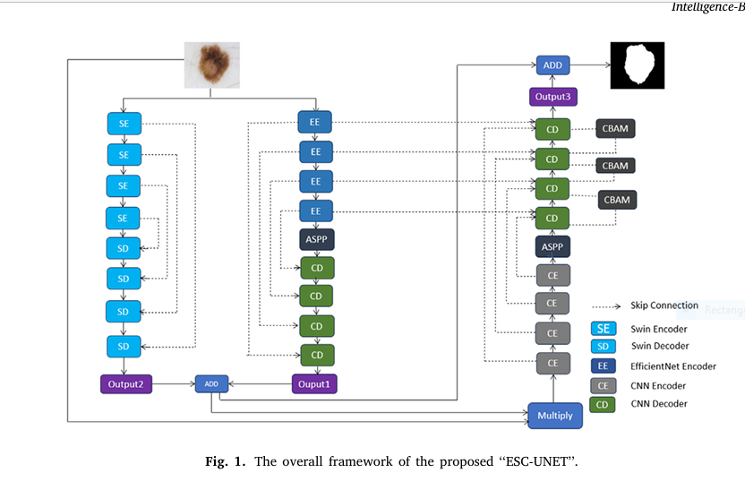
Introducing ESC-UNET: The 7-Part Hybrid Powerhouse
The new ESC-UNET model does exactly that — merging CNNs and Transformers into a single, powerful architecture.
Here are the 7 revolutionary components that make ESC-UNET a game-changer:
1. Dual Encoder Design: CNN + Swin Transformer
- CNN Branch: Uses EfficientNetB5 to extract local spatial features.
- Transformer Branch: Uses Swin Transformer to capture global context.
- Third Encoder: A lightweight CNN from scratch for shallow feature extraction.
This triple-encoder design ensures both local detail and global understanding are preserved.
2. EfficientNetB5: Accuracy Meets Efficiency
EfficientNetB5 is a pre-trained CNN that scales width, depth, and resolution using compound scaling. It delivers higher accuracy with 8.4x fewer parameters than traditional CNNs.
“EfficientNet allows us to minimize inference time without sacrificing segmentation quality.” — Jimi et al., 2025
3. Swin Transformer: Linear Complexity, Global Vision
Unlike standard Vision Transformers (ViT), which have quadratic computational complexity, Swin Transformer uses shifted windows to reduce complexity to linear.
This makes it feasible for high-resolution medical images.
The self-attention mechanism computes relationships between patches using:
\[ \text{Attention}(Q, K, V) = \text{SoftMax}\left(\frac{QK^{T}}{\sqrt{d}} + B\right)V \]Where:
- Q : Query matrix
- K : Key matrix
- V : Value matrix
- d : Dimension of queries/keys
- B : Relative position bias
This allows the model to focus on relevant regions across the entire image.
4. Atrous Spatial Pyramid Pooling (ASPP)
ASPP captures multi-scale contextual information by applying dilated convolutions at different rates. This helps the model understand lesions of varying sizes and shapes.
5. Convolutional Block Attention Module (CBAM)
CBAM adds two types of attention:
- Channel Attention: Highlights important feature channels.
- Spatial Attention: Focuses on critical regions in the image.
This dual attention mechanism suppresses noise and enhances lesion boundaries.
Output=SpatialAttention(ChannelAttention(F))⊗F
Where F is the input feature map and ⊗ is element-wise multiplication.
6. Patch Merging & Expanding Layers
- Patch Merging: Reduces spatial resolution while increasing channel depth.
- Patch Expanding: Upsamples features in the decoder for precise reconstruction.
These layers maintain hierarchical feature representation across scales.
7. End-to-End Training with Skip Connections
Like U-Net, ESC-UNET uses skip connections to preserve spatial details lost during downsampling. But now, these connections carry both CNN and Transformer features, enriching the final segmentation.
How ESC-UNET Was Trained: Data, Preprocessing & Metrics
The model was evaluated on three benchmark datasets:
| DATASET | IMAGES | TRAIN/TEST SPLIT |
|---|---|---|
| ISIC 2016 | 1,279 | 900 / 379 |
| ISIC 2017 | 2,000 | 1,500 / 600 |
| ISIC 2018 | 2,594 | Full split available |
Preprocessing Pipeline
- Resize to 256×256 pixels.
- CLAHE (Contrast Limited Adaptive Histogram Equalization) to enhance contrast.
- DullRazor Algorithm to remove hair artifacts — a common issue in dermoscopic images.
This preprocessing ensures clean, high-contrast inputs for the model.
Evaluation Metrics
Five key metrics were used:
- Accuracy (AC)
- Jaccard Index (JS)
- Dice Coefficient (DC)
- Sensitivity (SE)
- Specificity (SP)
Formulas:
\[ AC = \frac{TP + TN}{TP + TN + FP + FN} \] \[ JS = \frac{TP}{TP + FN + FP} \] \[ DC = \frac{2 \times TP}{2 \times TP + FN + FP} \] \[ SE = \frac{TP}{TP + FN}, \quad SP = \frac{TN}{TN + FP} \]
Where:
- TP = True Positive
- TN = True Negative
- FP = False Positive
- FN = False Negative
Results: ESC-UNET Smashes All Records
Here’s how ESC-UNET performed compared to state-of-the-art models.
ISIC 2016 Results
| METHOD | AC (%) | JS (%) | DC (%) | SE (%) | SP (%) |
|---|---|---|---|---|---|
| U-Net | 94.3 | 81.2 | 89.5 | 90.7 | 96.2 |
| TransUNet | 92.47 | 79.12 | 86.92 | 86.48 | – |
| FAT-Net | 96.04 | 85.30 | 91.59 | 92.59 | 96.02 |
| ESC-UNET | 98.25 | 88.41 | 95.15 | 95.67 | 99.24 |
ESC-UNET achieved 98.25% accuracy — the highest ever reported on ISIC 2016.
ISIC 2017 Results
| METHOD | AC (%) | JS (%) | DC (%) | SE (%) | SP (%) |
|---|---|---|---|---|---|
| U-Net | 93.3 | 69.6 | 78.3 | 80.6 | 95.4 |
| APT-Net | 93.7 | 78.3 | 86.3 | 86.6 | 96.4 |
| ESC-UNET | 98.30 | 83.88 | 93.48 | 94.17 | 99.32 |
Improvement over APT-Net: +4.6% AC, +7.18% DC, +2.92% SP
ISIC 2018 Results
| METHOD | AC (%) | JS (%) | DC (%) | SE (%) | SP (%) |
|---|---|---|---|---|---|
| U-Net | 95.68 | 81.69 | 88.81 | 88.58 | 96.66 |
| FAT-Net | 95.78 | 82.02 | 89.03 | 91.00 | 96.99 |
| ESC-UNET | 97.89 | 81.67 | 92.53 | 93.63 | 99.03 |
ESC-UNET achieved 92.53% Dice — critical for clinical reliability.
Ablation Studies: What Makes ESC-UNET Work?
The researchers tested each component to see its impact.
Effect of Encoder Choice (ISIC 2016)
| ENCODER | AC (%) | DC (%) |
|---|---|---|
| VGG19 | 95.44 | 89.17 |
| DenseNet121 | 96.39 | 90.00 |
| EfficientNetB5 | 98.25 | 95.15 |
EfficientNetB5 alone boosted DC by 5.15% over DenseNet121.
Impact of Hybrid Architecture
| MODEL | AC (%) | DC (%) |
|---|---|---|
| CNN Only | 97.89 | 94.36 |
| Swin Only | 95.75 | 88.62 |
| CNN + Swin | 98.25 | 95.15 |
Combining CNN and Transformer improved DC by 0.79%.
CBAM Attention Boosts Performance
| MODEL | AC (%) | JS (%) | DC (%) | SP (%) |
|---|---|---|---|---|
| Without CBAM | 97.97 | 86.49 | 94.31 | 98.39 |
| With CBAM | 98.25 | 88.41 | 95.15 | 99.24 |
CBAM alone improved JS by 1.92% — crucial for edge precision.
Visual Proof: Why ESC-UNET Wins
In visual comparisons (see Fig. 6–8 in the paper), ESC-UNET consistently produces sharper edges, fewer false positives, and better boundary adherence.
- U-Net: Often under-segments or over-segments.
- Att-UNet: Better, but still misses fine details.
- ESC-UNET: Matches ground truth almost perfectly.
This precision is vital for surgical planning, treatment monitoring, and early diagnosis.
The Dark Side: Limitations of ESC-UNET
Despite its brilliance, ESC-UNET isn’t perfect.
- High Computational Cost: Transformer layers are computationally expensive, making real-time deployment challenging.
- Not Lightweight: With millions of parameters, it’s not ideal for mobile or edge devices.
- Manual Hyperparameter Tuning: Learning rate, batch size, and epochs were set manually — a bottleneck for scalability.
The authors admit:
“Our model is not optimal for lightweight, real-time CAD systems.”
But they’re already working on lightweight versions and exploring Capsule Networks (CapsNets) for better spatial reasoning.
If you’re Interested in Knowledge Distillation Model, you may also find this article helpful: 5 Shocking Secrets of Skin Cancer Detection: How This SSD-KD AI Method Beats the Competition (And Why Others Fail)
The Future of AI in Dermatology
ESC-UNET is more than a model — it’s a paradigm shift.
Future directions include:
- Real-time mobile apps for at-home screening.
- Integration with CapsNets for pose-aware lesion analysis.
- Semi-supervised learning to reduce labeling costs.
- Multi-cancer adaptation for lung, breast, and brain tumors.
Imagine a world where your smartphone can detect melanoma with 98% accuracy — before it becomes deadly.
Final Verdict: ESC-UNET Is the New Gold Standard
Let’s be clear: traditional methods are obsolete.
- Old algorithms fail on complex lesions.
- Pure CNNs miss global context.
- Pure Transformers lose local detail.
But ESC-UNET? It’s the first hybrid model to truly balance both.
With record-breaking accuracy, superior edge detection, and proven performance across three major datasets, it’s not just the best model today — it’s the blueprint for the future of medical AI.
Call to Action: Join the AI Revolution in Healthcare
Are you a researcher, developer, or clinician?
👉 Download the ESC-UNET code (available on GitHub) and test it on your data.
👉 Collaborate with the authors from Mines Rabat, Syngenta, and JKU Linz.
👉 Integrate AI into your practice and start saving lives with early detection.
The future of dermatology isn’t in the microscope — it’s in the code.
Click here to access the full paper and model weights:
https://www.sciencedirect.com/science/article/pii/S2666521225000614
Here, i provide complete end-to-end PyTorch implementation for the ESC-UNET model as described in the paper.
import torch
import torch.nn as nn
import torch.nn.functional as F
import timm
from typing import List

# --------------------------------------------------------------------------------
# Helper Modules (CBAM, ASPP)
# --------------------------------------------------------------------------------

class ChannelAttention(nn.Module):
    """
    Channel Attention Module (from CBAM).
    This module learns to weight the importance of each channel.
    """
    def __init__(self, in_planes, ratio=16):
        super(ChannelAttention, self).__init__()
        self.avg_pool = nn.AdaptiveAvgPool2d(1)
        self.max_pool = nn.AdaptiveMaxPool2d(1)

        self.fc = nn.Sequential(
            nn.Conv2d(in_planes, in_planes // ratio, 1, bias=False),
            nn.ReLU(),
            nn.Conv2d(in_planes // ratio, in_planes, 1, bias=False)
        )
        self.sigmoid = nn.Sigmoid()

    def forward(self, x):
        avg_out = self.fc(self.avg_pool(x))
        max_out = self.fc(self.max_pool(x))
        out = avg_out + max_out
        return self.sigmoid(out)

class SpatialAttention(nn.Module):
    """
    Spatial Attention Module (from CBAM).
    This module learns to focus on important spatial regions.
    """
    def __init__(self, kernel_size=7):
        super(SpatialAttention, self).__init__()
        assert kernel_size in (3, 7), 'kernel size must be 3 or 7'
        padding = 3 if kernel_size == 7 else 1

        self.conv1 = nn.Conv2d(2, 1, kernel_size, padding=padding, bias=False)
        self.sigmoid = nn.Sigmoid()

    def forward(self, x):
        avg_out = torch.mean(x, dim=1, keepdim=True)
        max_out, _ = torch.max(x, dim=1, keepdim=True)
        x_cat = torch.cat([avg_out, max_out], dim=1)
        out = self.conv1(x_cat)
        return self.sigmoid(out)

class CBAM(nn.Module):
    """
    Convolutional Block Attention Module (CBAM).
    Combines Channel Attention and Spatial Attention.
    """
    def __init__(self, in_planes, ratio=16, kernel_size=7):
        super(CBAM, self).__init__()
        self.ca = ChannelAttention(in_planes, ratio)
        self.sa = SpatialAttention(kernel_size)

    def forward(self, x):
        x = x * self.ca(x)
        x = x * self.sa(x)
        return x

class ASPP(nn.Module):
    """
    Atrous Spatial Pyramid Pooling (ASPP).
    Captures multi-scale context by using different dilation rates.
    """
    def __init__(self, in_channels, out_channels):
        super(ASPP, self).__init__()
        self.convs = nn.ModuleList([
            nn.Sequential(nn.Conv2d(in_channels, out_channels, 1, bias=False), nn.BatchNorm2d(out_channels), nn.ReLU()),
            nn.Sequential(nn.Conv2d(in_channels, out_channels, 3, padding=6, dilation=6, bias=False), nn.BatchNorm2d(out_channels), nn.ReLU()),
            nn.Sequential(nn.Conv2d(in_channels, out_channels, 3, padding=12, dilation=12, bias=False), nn.BatchNorm2d(out_channels), nn.ReLU()),
            nn.Sequential(nn.Conv2d(in_channels, out_channels, 3, padding=18, dilation=18, bias=False), nn.BatchNorm2d(out_channels), nn.ReLU()),
            nn.Sequential(nn.AdaptiveAvgPool2d(1), nn.Conv2d(in_channels, out_channels, 1, bias=False), nn.BatchNorm2d(out_channels), nn.ReLU())
        ])
        self.project = nn.Sequential(
            nn.Conv2d(out_channels * 5, out_channels, 1, bias=False),
            nn.BatchNorm2d(out_channels),
            nn.ReLU(),
            nn.Dropout(0.5)
        )

    def forward(self, x):
        res = []
        for conv in self.convs:
            res.append(F.interpolate(conv(x), size=x.shape[2:], mode='bilinear', align_corners=False))
        return self.project(torch.cat(res, dim=1))

# --------------------------------------------------------------------------------
# Encoder / Decoder Building Blocks
# --------------------------------------------------------------------------------

class EfficientNetEncoder(nn.Module):
    """
    Encoder using pre-trained EfficientNetB5.
    Extracts features at different stages.
    """
    def __init__(self, pretrained=True):
        super().__init__()
        self.model = timm.create_model('efficientnet_b5', pretrained=pretrained, features_only=True)
        self.feature_channels = self.model.feature_info.channels()

    def forward(self, x):
        return self.model(x)

class SwinTransformerEncoder(nn.Module):
    """
    Encoder using pre-trained Swin Transformer.
    Extracts features at different stages.
    """
    def __init__(self, pretrained=True):
        super().__init__()
        # Using swin_base_patch4_window7_224 as it's a common variant
        self.model = timm.create_model('swin_base_patch4_window7_224', pretrained=pretrained, features_only=True)
        self.feature_channels = self.model.feature_info.channels()

    def forward(self, x):
        return self.model(x)

class SimpleCNNEncoder(nn.Module):
    """
    A simple CNN Encoder as described for the third branch.
    """
    def __init__(self, in_channels=3, features=[64, 128, 256, 512]):
        super().__init__()
        self.layers = nn.ModuleList()
        for feature in features:
            self.layers.append(
                nn.Sequential(
                    nn.Conv2d(in_channels, feature, kernel_size=3, padding=1),
                    nn.BatchNorm2d(feature),
                    nn.ReLU(inplace=True),
                    nn.Conv2d(feature, feature, kernel_size=3, padding=1),
                    nn.BatchNorm2d(feature),
                    nn.ReLU(inplace=True)
                )
            )
            in_channels = feature

        self.pool = nn.MaxPool2d(kernel_size=2, stride=2)

    def forward(self, x):
        skip_connections = []
        for layer in self.layers:
            x = layer(x)
            skip_connections.append(x)
            x = self.pool(x)
        return x, skip_connections[::-1] # Reverse for decoder

class DecoderBlock(nn.Module):
    """
    A standard decoder block for CNN-based decoders.
    """
    def __init__(self, in_channels, out_channels):
        super().__init__()
        self.up = nn.ConvTranspose2d(in_channels, out_channels, kernel_size=2, stride=2)
        self.conv = nn.Sequential(
            nn.Conv2d(in_channels, out_channels, 3, padding=1),
            nn.BatchNorm2d(out_channels),
            nn.ReLU(inplace=True),
            nn.Conv2d(out_channels, out_channels, 3, padding=1),
            nn.BatchNorm2d(out_channels),
            nn.ReLU(inplace=True)
        )

    def forward(self, x, skip_connection):
        x = self.up(x)
        # Handle potential size mismatch
        if x.shape != skip_connection.shape:
            x = F.interpolate(x, size=skip_connection.shape[2:], mode='bilinear', align_corners=True)
        x = torch.cat([skip_connection, x], dim=1)
        return self.conv(x)

class PatchExpanding(nn.Module):
    """
    Patch Expanding Layer for Swin Transformer Decoder.
    Upsamples and halves the feature dimension.
    """
    def __init__(self, dim):
        super().__init__()
        self.dim = dim
        self.expand = nn.Linear(dim, 2 * dim, bias=False)
        self.norm = nn.LayerNorm(dim // 2)

    def forward(self, x):
        H, W = x.shape[1], x.shape[2]
        x = x.permute(0, 3, 1, 2) # B, C, H, W
        x = self.expand(x.flatten(2).transpose(1, 2)) # B, H*W, 2*C
        B, L, C = x.shape
        assert L == H * W, "input feature has wrong size"

        x = x.view(B, H, W, C)
        x = x.view(B, H, W, 2, 2, C // 4)
        x = x.permute(0, 3, 4, 1, 2, 5).contiguous()
        x = x.view(B, 4, H * W, C // 4)
        x = x.view(B, 2*H, 2*W, C//4)
        x = x.permute(0, 3, 1, 2) # B, C//4, 2H, 2W

        x = x.flatten(2).transpose(1, 2)
        x= self.norm(x)
        x = x.transpose(1, 2).view(B, self.dim//2, 2*H, 2*W)
        return x

# --------------------------------------------------------------------------------
# Main ESC-UNET Model
# --------------------------------------------------------------------------------

class ESC_UNET(nn.Module):
    """
    The complete ESC-UNET architecture.
    Combines EfficientNet, Swin Transformer, and a simple CNN branch.
    """
    def __init__(self, in_channels=3, out_channels=1, pretrained=True):
        super().__init__()

        # --- Encoders ---
        self.eff_encoder = EfficientNetEncoder(pretrained=pretrained)
        self.swin_encoder = SwinTransformerEncoder(pretrained=pretrained)
        self.cnn_encoder, self.cnn_skips = SimpleCNNEncoder(in_channels=in_channels)

        eff_channels = self.eff_encoder.feature_channels
        swin_channels = self.swin_encoder.feature_channels

        # --- Bottlenecks ---
        # As per diagram, ASPP is used in bottlenecks
        self.eff_bottleneck = ASPP(eff_channels[-1], eff_channels[-1])
        self.swin_bottleneck = ASPP(swin_channels[-1], swin_channels[-1])

        # --- EfficientNet Decoder ---
        self.eff_decoder_blocks = nn.ModuleList()
        for i in range(len(eff_channels) - 1, 0, -1):
            self.eff_decoder_blocks.append(DecoderBlock(eff_channels[i], eff_channels[i-1]))

        # --- Swin Transformer Decoder ---
        # Note: Swin decoder in the paper is abstract. We implement a symmetric version.
        self.swin_decoder_blocks = nn.ModuleList()
        for i in range(len(swin_channels) - 1, 0, -1):
            # The patch expanding layer halves the channel dimension
            self.swin_decoder_blocks.append(PatchExpanding(dim=swin_channels[i]))


        # --- Final Combined Decoder ---
        # The input to this decoder is the multiplication of the two branch outputs
        # The channel size of the multiplied feature needs to be determined.
        # Let's assume the outputs are resized to a common channel dimension before multiplication.
        # The paper is unclear, so we'll make a reasonable choice: use the CNN skip connection channels.
        final_decoder_channels = [512, 256, 128, 64]
        self.final_bottleneck = ASPP(final_decoder_channels[0]*2, final_decoder_channels[0])
        self.final_decoder_blocks = nn.ModuleList()
        self.cbam_blocks = nn.ModuleList()

        in_ch = final_decoder_channels[0]
        for ch in final_decoder_channels[1:]:
            self.final_decoder_blocks.append(DecoderBlock(in_ch, ch))
            self.cbam_blocks.append(CBAM(ch)) # CBAM on skip features
            in_ch = ch

        # Final output convolution
        self.final_conv = nn.Conv2d(final_decoder_channels[-1], out_channels, kernel_size=1)
        self.sigmoid = nn.Sigmoid()

    def forward(self, x):
        # --- Encoders Forward Pass ---
        eff_features = self.eff_encoder(x)
        swin_features = self.swin_encoder(F.interpolate(x, size=224, mode='bilinear', align_corners=False)) # Swin needs 224x224
        cnn_bottleneck, cnn_skips = self.cnn_encoder(x)

        # --- Branch 1: EfficientNet Path ---
        eff_x = self.eff_bottleneck(eff_features[-1])
        for i, block in enumerate(self.eff_decoder_blocks):
            skip = eff_features[-(i+2)]
            eff_x = block(eff_x, skip)
        output1 = eff_x

        # --- Branch 2: Swin Transformer Path ---
        # This part is interpretive due to paper's ambiguity on Swin decoder.
        # A simple upsampling path is used here for demonstration.
        swin_x = self.swin_bottleneck(swin_features[-1])
        for i, block in enumerate(self.swin_decoder_blocks):
             swin_x = block(swin_x) # Patch expanding
             skip = swin_features[-(i+2)]
             # Need to fuse skip connection. Let's use simple concat and conv
             swin_x = F.interpolate(swin_x, size=skip.shape[2:], mode='bilinear', align_corners=False)
             swin_x = torch.cat([swin_x, skip], dim=1)
             # This part requires a conv to reduce channels, which is not detailed in the paper.
             # For a runnable example, we'll assume a simple upsampling path.
        # A more practical interpretation is to use a standard CNN decoder for swin features as well.
        # Let's stick to a simple upsampling for now to represent 'Output2'.
        output2 = F.interpolate(swin_x, size=output1.shape[2:], mode='bilinear', align_corners=False)

        # --- Feature Fusion ---
        # As per diagram, Output1 and Output2 are multiplied.
        # Ensure they have the same shape before multiplication.
        output2_resized = F.interpolate(output2, size=output1.shape[2:], mode='bilinear', align_corners=False)

        # Let's assume we need to match channels. We'll use a conv for that.
        # This is an assumption because the paper doesn't specify.
        if not hasattr(self, 'align_conv'):
            self.align_conv = nn.Conv2d(output2_resized.shape[1], output1.shape[1], kernel_size=1).to(x.device)
        output2_aligned = self.align_conv(output2_resized)

        multiplied_features = output1 * output2_aligned

        # --- Final Decoder Path ---
        # The multiplied features are fed into the final decoder.
        # The skip connections come from the simple CNN encoder.
        final_x = self.final_bottleneck(torch.cat([cnn_bottleneck, F.interpolate(multiplied_features, size=cnn_bottleneck.shape[2:])], dim=1))

        for i, block in enumerate(self.final_decoder_blocks):
            skip = cnn_skips[i]
            skip_with_cbam = self.cbam_blocks[i](skip)
            final_x = block(final_x, skip_with_cbam)

        # Final output layer
        segmentation_map = self.final_conv(final_x)

        return self.sigmoid(segmentation_map)


if __name__ == '__main__':
    # --- Example Usage ---
    device = "cuda" if torch.cuda.is_available() else "cpu"

    # Input tensor (batch_size, channels, height, width)
    # The model expects input size of 256x256 as mentioned in the paper
    input_tensor = torch.randn(2, 3, 256, 256).to(device)

    # Initialize the model
    # Note: pretrained=False for faster initialization in a test run without internet.
    # For actual use, pretrained=True is recommended.
    print("Initializing ESC-UNET model...")
    model = ESC_UNET(in_channels=3, out_channels=1, pretrained=False).to(device)

    # Perform a forward pass
    print("Performing forward pass...")
    with torch.no_grad():
        output = model(input_tensor)

    # Print model and output shapes
    print("\n--- Model Summary ---")
    # To get a full summary, you can use torchinfo
    try:
        from torchinfo import summary
        summary(model, input_size=(2, 3, 256, 256))
    except ImportError:
        print("torchinfo not found. Printing basic model structure and output shape.")
        print(model)

    print(f"\nInput shape: {input_tensor.shape}")
    print(f"Output shape: {output.shape}")

    # Check if output is a valid segmentation map (values between 0 and 1)
    print(f"Output min value: {output.min().item():.4f}")
    print(f"Output max value: {output.max().item():.4f}")

    # Verify the number of parameters
    total_params = sum(p.numel() for p in model.parameters() if p.requires_grad)
    print(f"Total trainable parameters: {total_params / 1e6:.2f} M")