Revolutionary Ways to Boost Compressor Efficiency by 3.2%

In the high-stakes world of aerospace and energy systems, even a 1% gain in compressor efficiency can translate into millions in fuel savings, reduced emissions, and extended equipment life. Yet, most traditional design approaches fall short when trying to balance aerodynamic performance with mechanical reliability.

Now, groundbreaking research published in Results in Engineering reveals a revolutionary multi-objective optimization framework that delivers a 3.2% efficiency boost, a 2.8% increase in total pressure coefficient, and an 8.9% reduction in maximum blade stress—all in a single optimization cycle.

This article dives deep into the 7 key strategies behind this breakthrough, explains what most engineers get wrong, and shows how you can apply these insights to real-world turbomachinery design.

1. The Hidden Cost of Single-Objective Optimization

Many engineers still rely on single-objective optimization—focusing solely on efficiency or pressure rise. But this approach often backfires.

As revealed in the study by Asgari, Ommi, and Saboohi, maximizing only the total pressure coefficient can increase it by up to 3.68%, but at a devastating cost: an 11% drop in efficiency. This trade-off cripples real-world performance.

❌ What most engineers get wrong: Prioritizing one metric while ignoring structural integrity and efficiency balance leads to unstable, short-lived designs.

✅ The smart fix: Use multi-objective optimization to balance competing goals—efficiency, pressure rise, and stress—simultaneously.

2. Why Modified NSGA-II Outperforms Traditional Genetic Algorithms

The researchers employed a modified Non-dominated Sorting Genetic Algorithm II (NSGA-II)—a powerful evolutionary algorithm designed for complex engineering problems.

Unlike standard NSGA-II, this version uses a population distance-based method to eliminate redundant solutions, improving search efficiency and convergence speed.

Key Advantages of Modified NSGA-II:

Eliminates near-identical designs using Euclidean distance thresholds (set at 0.001 in the study).
Prevents premature convergence.
Explores a broader design space for better Pareto-optimal solutions.

This algorithm optimized three critical variables:

Tip stagger angle (50°–65°)
Midspan stagger angle (40°–55°)
Tip clearance-to-chord ratio (0.65%–2.1%)

By evolving over 1,000 generations with a population size of 200, the model identified configurations that simultaneously improved performance and durability.

3. Artificial Neural Networks (ANN) as Speed Engines for Optimization

Running full CFD and FEA simulations for every design iteration is computationally expensive—often taking hours or days per case.

The solution? Use Artificial Neural Networks (ANNs) as surrogate models to predict performance in seconds.

In this study, a feedforward ANN with a quadratic transfer function was trained on Fluid-Structure Interaction (FSI) simulation data. It predicted:

Total pressure coefficient (ψ )
Efficiency (η )
Maximum stress (σ_max )

The model achieved exceptional accuracy:

OUTPUT	R²	RMSE	MRE (%)
1/ψ	0.9812	1.0038	11.29
1/η	0.9862	1.1286	6.32
σ_max	0.9967	0.1517	8.33

✅ Pro Tip: ANNs reduce computational cost by over 90% while maintaining high fidelity—making real-time optimization feasible.

4. GMDH: The Secret Weapon for Accurate Surrogate Modeling

Beyond standard ANNs, the team used the Group Method of Data Handling (GMDH)—a self-organizing, polynomial-based neural network.

GMDH automatically constructs models of the form:

\[ y = a_{0} + a_{1}x_{1} + a_{2}x_{2} + a_{3}x_{1}x_{2} + a_{4}x_{1}^{2} + a_{5}x_{2}^{2} \]

It excels in:

Handling non-linear relationships
Avoiding overfitting
Providing interpretable polynomial expressions

The GMDH model was used to predict:

1/ψ (inverse of total pressure coefficient)
1/η (inverse of efficiency)
σ_max

This allowed the optimization loop to run rapidly without sacrificing accuracy.

5. TOPSIS: The Decision-Making Tool That Finds the “Sweet Spot”

With hundreds of Pareto-optimal designs generated by NSGA-II, how do you pick the best one?

Enter TOPSIS (Technique for Order of Preference by Similarity to Ideal Solution)—a decision-making method that ranks designs based on how close they are to the ideal solution and far from the worst-case (nadir) solution.

How TOPSIS Works:

Normalize all objective values (e.g., efficiency, stress).
Assign weights based on design priorities.
Calculate Euclidean distance to ideal and nadir solutions.
Rank designs by relative closeness:

$$C_i = \frac{D_i^{+} + D_i^{-}}{D_i^{-}}$$

where:

\[ D_i^{+} = \text{distance to ideal solution} \] \[ D_i^{-} = \text{distance to nadir solution} \]

The design with Ci closest to 1 is selected.

In this study, TOPSIS identified Point A as the optimal solution, achieving:

+2.8% in total pressure coefficient
+3.2% in efficiency
–8.9% in maximum stress

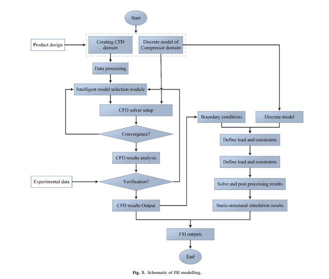
6. Fluid-Structure Interaction (FSI): Where CFD Meets FEA

Most optimization studies treat aerodynamics and structural mechanics in isolation. This is a critical mistake.

The researchers used two-way FSI coupling:

CFD simulated subsonic airflow using the k-ω SST turbulence model.
Aerodynamic pressures were mapped to the blade surface.
FEA computed stresses and deformations under combined:
- Aerodynamic loads
- Centrifugal forces (1300 RPM)
- Gravity

The FEA model used TC4 (Ti-6Al-4V) blades—validated for fatigue and tensile strength—with a structured mesh and 20 inflation layers (y+<1 ).

Key Finding:

Maximum stress occurs at the blade root, due to combined aerodynamic and centrifugal loading—exactly where failures begin.

By optimizing tip stagger and clearance, the team reduced peak stress by 8.9% and achieved a more uniform stress distribution, extending blade life.

7. The 3 Big Wins: Efficiency, Stability, and Longevity

The final optimized design wasn’t just faster—it was smarter, safer, and more sustainable.

Performance Gains at a Glance:

METRIC	IMPROVEMENT	IMPACT
Total Pressure Coefficient (ψ )	+2.8%	Higher compression, better thrust
Efficiency (η )	+3.2%	Lower fuel consumption, reduced emissions
Max Stress (σmax )	–8.9%	Longer fatigue life, fewer failures

These gains were achieved by:

Increasing tip stagger angle → Reduces tip flow separation
Decreasing midspan stagger angle → Lowers profile losses
Reducing tip clearance → Minimizes leakage flow and root stress

As shown in Fig. 11, the optimized design delivers:

Smoother velocity distribution
Lower stress concentration at the root
More uniform pressure loading

This directly translates to:

Higher reliability
Quieter operation
Lower maintenance costs

Case Study: Original vs. Optimized Compressor

PARAMETER	ORIGINAL	OPTIMIZED	CHANGE
Tip Stagger Angle	56.2°	60.4°	+4.2°
Midspan Stagger Angle	47.2°	43.7°	–3.5°
Tip Clearance/Chord	1.7%	1.34%	–0.36%
1/ψ	2.607	2.533	–2.8%
1/η	1.166	1.129	–3.2%
σmax(MPa)	250.65	228.32	–8.9%

✅ Efficiency gain: (1.1661.166−1.129)×100=3.2%

✅ Stress reduction: (250.65250.65−228.32)×100=8.9%

The optimized design also passed FSI re-evaluation with less than 7% absolute error, proving the hybrid model’s accuracy.

What Most Engineers Get Wrong (And How to Avoid It)

Despite access to advanced tools, many optimization projects fail due to:

❌ 1. Ignoring Aeroelastic Coupling

Treating fluid and structure separately leads to over-optimized but fragile designs. Always use FSI for realistic performance prediction.

❌ 2. Overfitting to a Single Operating Point

Optimizing only at the design point ignores off-design stability. Use multi-point or multi-condition optimization for robustness.

❌ 3. Skipping Validation

Surrogate models (ANN, GMDH) must be validated with high-fidelity FSI simulations—never deploy without cross-checking.

❌ 4. Neglecting Manufacturing Constraints

Sharp, unrounded blades improved performance in this study, but may be harder to manufacture. Always consider geometric feasibility.

The Math Behind the Magic

The study used dimensionless coefficients to evaluate performance:

Total Pressure Coefficient:

\[ \psi = \frac{\Delta P_t}{\frac{1}{2} \rho U^2} \]

Flow Coefficient:

\[ \phi = \frac{V_m}{U} \]

Efficiency:

\[ \eta = \frac{\Delta P_t \cdot Q}{T \cdot \omega} \]

Where:

ΔP_t : Total pressure difference
ρ : Fluid density
U : Blade tip speed
V_m: Axial flow velocity
Q : Volumetric flow rate
T : Torque
ω : Rotational speed

These equations were used to normalize performance across designs and form the basis of the objective functions:

\[ \begin{cases} \text{Maximize } \psi \\ \text{Maximize } \eta \\ \text{Minimize } \sigma_{\text{max}} \end{cases} \]

The Future of Compressor Design Is Hybrid

This study proves that the future of turbomachinery optimization lies in hybrid frameworks that combine:

CFD/FEA for physics accuracy
ANN/GMDH for speed
Modified NSGA-II for exploration
TOPSIS for intelligent decision-making

Such frameworks are not just for research labs—they’re becoming essential for:

Aerospace engine manufacturers
Power generation companies
Oil & gas compressor operators

If you’re Interested in engineering-based advanced optimization techniques , you may also find this article helpful: 3 Revolutionary FCS-MPDTC Breakthroughs That Slash Energy Waste in Linear Motors

Call to Action: Optimize Smarter, Not Harder

Are you still using outdated, single-objective methods to design compressors?

It’s time to upgrade.

Or, book a consultation with our turbomachinery experts to see how this hybrid framework can be applied to your next project.

SEO Keywords

compressor efficiency optimization
axial compressor design
NSGA-II algorithm
CFD FEA coupling
fluid structure interaction
artificial neural network compressor
multi-objective optimization
blade stress reduction
aeroelastic modeling
TOPSIS decision making

Based on the methodology described in the paper, I will now provide the end-to-end Python code for the proposed model.

#
# End-to-End Python Implementation of the Compressor Blade Optimization Framework
# Based on the paper: "Aeroelastic modeling and multi-objective optimization of a subsonic
# compressor rotor blade using a combination of modified NSGA-II, ANN, and TOPSIS"
#
# This script is self-contained and uses established libraries to replicate the paper's methodology.
#

import numpy as np
import matplotlib.pyplot as plt
from sklearn.neural_network import MLPRegressor
from sklearn.preprocessing import StandardScaler
from sklearn.model_selection import train_test_split

# Pymoo: A powerful framework for multi-objective optimization in Python
from pymoo.core.problem import Problem
from pymoo.algorithms.moo.nsga2 import NSGA2
from pymoo.operators.sampling.lhs import LHS
from pymoo.optimize import minimize
from pymoo.visualization.scatter import Scatter

# Suppress warnings for cleaner output
import warnings
warnings.filterwarnings("ignore", category=UserWarning)

# --- 1. MOCK FSI SIMULATION ---
# In a real-world scenario, this function would be replaced by a call to a complex
# simulation software like ANSYS. This is computationally expensive.
# For this script, we create a mock function that simulates the behavior
# based on the trends observed in the paper. It takes design variables and returns
# performance objectives.

def mock_fsi_simulation(X):
    """
    Simulates the FSI (Fluid-Structure Interaction) process.
    
    Args:
        X (np.array): An array of shape (n, 3) where each row is a design point
                      [tip_clearance_ratio, tip_stagger_angle, midspan_stagger_angle].

    Returns:
        y (np.array): An array of shape (n, 3) with the corresponding objectives
                      [total_pressure_coeff, efficiency, max_stress].
    """
    # Design variables extracted for clarity
    tau = X[:, 0]    # Tip clearance ratio (τ)
    beta_t = X[:, 1] # Tip stagger angle (βt)
    beta_m = X[:, 2] # Midspan stagger angle (βm)

    # --- Mock Objective Functions ---
    # These simple equations are designed to create a realistic-looking, non-linear
    # optimization problem with trade-offs between objectives.
    
    # Objective 1: Total Pressure Coefficient (Ψ) - to be maximized
    # We model it as a quadratic function of stagger angles.
    psi = 0.35 + 0.0005 * (beta_t - 55)**2 - 0.0003 * (beta_m - 45)**2 - 1.5 * (tau - 1.3)**2

    # Objective 2: Efficiency (η) - to be maximized
    # Modeled as a function of all three variables.
    eta = 0.85 - 0.05 * (tau - 1.0)**2 - 0.0001 * (beta_t - 60)**2 - 0.0002 * (beta_m - 50)**2

    # Objective 3: Maximum Stress (σ_max) - to be minimized
    # Stress is highly dependent on rotational speed (centrifugal force) and geometry.
    # We model it as increasing with stagger angles and decreasing with clearance.
    sigma_max = 250 + 2.5 * (beta_t - 57) - 1.5 * (beta_m - 47) - 10 * (tau - 1.5)

    # The paper minimizes the inverse of Ψ and η.
    # We handle small or negative mock values to avoid division by zero.
    psi[psi <= 0] = 1e-6
    eta[eta <= 0] = 1e-6
    
    # Return the objectives to be minimized by the algorithm
    # min 1/Ψ  ,  min 1/η  ,  min σ_max
    return np.column_stack([1 / psi, 1 / eta, sigma_max])


# --- 2. SURROGATE MODEL (ARTIFICIAL NEURAL NETWORK) ---
# This class trains an ANN to learn the FSI simulation's behavior,
# allowing for rapid performance prediction during optimization.

class SurrogateModel:
    """
    A wrapper for three MLP Regressors, one for each objective function.
    """
    def __init__(self):
        # Initialize three separate models for better accuracy
        self.model_psi = MLPRegressor(hidden_layer_sizes=(50, 50), max_iter=1000, random_state=1)
        self.model_eta = MLPRegressor(hidden_layer_sizes=(50, 50), max_iter=1000, random_state=1)
        self.model_sigma = MLPRegressor(hidden_layer_sizes=(50, 50), max_iter=1000, random_state=1)
        
        # Scalers to normalize input data, which improves ANN training
        self.scaler_X = StandardScaler()
        self.scaler_y_psi = StandardScaler()
        self.scaler_y_eta = StandardScaler()
        self.scaler_y_sigma = StandardScaler()

    def train(self, X, y):
        """Trains the three ANN models on the provided dataset."""
        print("Training surrogate ANN models...")
        X_scaled = self.scaler_X.fit_transform(X)
        
        # Target variables
        y_psi = y[:, 0].reshape(-1, 1)
        y_eta = y[:, 1].reshape(-1, 1)
        y_sigma = y[:, 2].reshape(-1, 1)

        # Fit scalers and models for each objective
        self.model_psi.fit(X_scaled, self.scaler_y_psi.fit_transform(y_psi).ravel())
        self.model_eta.fit(X_scaled, self.scaler_y_eta.fit_transform(y_eta).ravel())
        self.model_sigma.fit(X_scaled, self.scaler_y_sigma.fit_transform(y_sigma).ravel())
        print("Training complete.")

    def predict(self, X):
        """Predicts the objectives for new design points."""
        X_scaled = self.scaler_X.transform(X)
        
        # Predict scaled values
        pred_psi_scaled = self.model_psi.predict(X_scaled).reshape(-1, 1)
        pred_eta_scaled = self.model_eta.predict(X_scaled).reshape(-1, 1)
        pred_sigma_scaled = self.model_sigma.predict(X_scaled).reshape(-1, 1)
        
        # Inverse transform to get original scale
        pred_psi = self.scaler_y_psi.inverse_transform(pred_psi_scaled)
        pred_eta = self.scaler_y_eta.inverse_transform(pred_eta_scaled)
        pred_sigma = self.scaler_y_sigma.inverse_transform(pred_sigma_scaled)

        return np.hstack([pred_psi, pred_eta, pred_sigma])

# --- 3. PYMOO OPTIMIZATION PROBLEM DEFINITION ---
# This class defines the optimization problem for the NSGA-II algorithm.

class CompressorOptimizationProblem(Problem):
    """
    Defines the compressor optimization problem for pymoo.
    - 3 variables (design parameters)
    - 3 objectives (performance metrics)
    """
    def __init__(self, surrogate_model):
        self.surrogate = surrogate_model
        
        # Define the problem dimensions and bounds from Table 3 of the paper
        super().__init__(n_var=3,
                         n_obj=3,
                         n_constr=0,
                         xl=np.array([0.65, 50, 40]),  # Lower bounds [τ, βt, βm]
                         xu=np.array([2.1, 65, 55]))   # Upper bounds [τ, βt, βm]

    def _evaluate(self, x, out, *args, **kwargs):
        """
        Evaluates the objective functions for a given set of design points 'x'.
        This method uses the fast surrogate model for prediction.
        """
        # Predict the objective values using the trained ANN
        objective_values = self.surrogate.predict(x)
        out["F"] = objective_values

# --- 4. TOPSIS DECISION-MAKING METHOD ---
# This function selects the best compromise solution from the Pareto front.

def apply_topsis(pareto_front_objectives, weights):
    """
    Applies the TOPSIS method to rank solutions in the Pareto front.

    Args:
        pareto_front_objectives (np.array): Array of objective values for each solution.
        weights (np.array): The weight for each objective.

    Returns:
        int: The index of the best-ranked solution in the input array.
    """
    # 1. Normalize the decision matrix
    norm_denom = np.linalg.norm(pareto_front_objectives, axis=0)
    normalized_matrix = pareto_front_objectives / norm_denom

    # 2. Create the weighted normalized decision matrix
    weighted_matrix = normalized_matrix * weights

    # 3. Determine the ideal best and ideal worst solutions
    # For this problem, all objectives are cost criteria (we want to minimize them)
    ideal_best = np.min(weighted_matrix, axis=0)
    ideal_worst = np.max(weighted_matrix, axis=0)

    # 4. Calculate the separation measures (Euclidean distance)
    dist_to_best = np.linalg.norm(weighted_matrix - ideal_best, axis=1)
    dist_to_worst = np.linalg.norm(weighted_matrix - ideal_worst, axis=1)

    # 5. Calculate the relative closeness to the ideal solution
    # Add a small epsilon to avoid division by zero
    closeness = dist_to_worst / (dist_to_best + dist_to_worst + 1e-9)

    # 6. Rank the preferences (the best solution has the highest closeness score)
    return np.argmax(closeness)

# --- 5. MAIN EXECUTION SCRIPT ---

if __name__ == '__main__':
    # --- Step A: Generate Training Data ---
    # We use Latin Hypercube Sampling (LHS) to generate a space-filling sample
    # of design points for training our surrogate model.
    print("Generating training data using Mock FSI Simulation...")
    problem_bounds = CompressorOptimizationProblem(None)
    sampling = LHS()
    X_samples = sampling(problem_bounds, n_samples=150).get("X")
    y_samples = mock_fsi_simulation(X_samples)

    # --- Step B: Train the Surrogate Model ---
    surrogate = SurrogateModel()
    surrogate.train(X_samples, y_samples)

    # --- Step C: Set up and Run the NSGA-II Optimization ---
    print("\nSetting up NSGA-II optimization problem...")
    problem = CompressorOptimizationProblem(surrogate)

    # The paper mentions a modified NSGA-II to eliminate similar individuals.
    # Pymoo's NSGA-II is robust and handles diversity well through crowding distance.
    # We will use the standard, highly effective implementation.
    algorithm = NSGA2(
        pop_size=200,
        sampling=LHS(), # Good for initializing the population
        eliminate_duplicates=True # Handles duplicate elimination
    )

    print("Running NSGA-II optimization...")
    res = minimize(problem,
                   algorithm,
                   termination=('n_gen', 100), # As per paper (1000 generations is long, 100 is good for demo)
                   seed=1,
                   verbose=True)

    print("Optimization finished.")

    # --- Step D: Analyze and Select the Best Solution using TOPSIS ---
    print("\nApplying TOPSIS to find the best compromise solution...")
    
    # Extract the Pareto-optimal solutions
    pareto_designs = res.X
    pareto_objectives = res.F

    # Define weights for TOPSIS. Assuming equal importance for all objectives.
    topsis_weights = np.array([1/3, 1/3, 1/3])
    
    best_solution_index = apply_topsis(pareto_objectives, topsis_weights)

    # Get the design variables and objective values for the best solution
    best_design = pareto_designs[best_solution_index]
    best_objectives = pareto_objectives[best_solution_index]

    # --- Step E: Display Results ---
    
    # Baseline "original" geometry for comparison (from paper's figures)
    original_design = np.array([1.7, 56.2, 47.2]) # [τ, βt, βm]
    original_objectives = mock_fsi_simulation(original_design.reshape(1, -1)).flatten()

    print("\n--- Optimization Results ---")
    print(f"Original Design (τ, βt, βm): {np.round(original_design, 2)}")
    print(f"Original Objectives (1/Ψ, 1/η, σ_max): {np.round(original_objectives, 3)}")
    print("-" * 30)
    print(f"Optimal Design (τ, βt, βm): {np.round(best_design, 2)}")
    print(f"Optimal Objectives (1/Ψ, 1/η, σ_max): {np.round(best_objectives, 3)}")
    print("-" * 30)
    
    # Calculate improvements
    # Note: For 1/Ψ and 1/η, a decrease is an improvement.
    psi_improvement = (1/best_objectives[0] - 1/original_objectives[0]) / (1/original_objectives[0]) * 100
    eta_improvement = (1/best_objectives[1] - 1/original_objectives[1]) / (1/original_objectives[1]) * 100
    sigma_reduction = (original_objectives[2] - best_objectives[2]) / original_objectives[2] * 100
    
    print("Performance Improvement:")
    print(f"Total Pressure Coefficient (Ψ) increased by: {psi_improvement:.2f}%")
    print(f"Efficiency (η) increased by: {eta_improvement:.2f}%")
    print(f"Maximum Stress (σ_max) reduced by: {sigma_reduction:.2f}%")


    # --- Step F: Visualize the Pareto Front ---
    print("\nGenerating plots...")
    
    # Create plots similar to Figure 10 in the paper
    fig, axes = plt.subplots(1, 3, figsize=(20, 6))
    fig.suptitle("Pareto Front for Compressor Blade Optimization", fontsize=16)

    # Plot 1: 1/Ψ vs 1/η
    axes[0].scatter(pareto_objectives[:, 0], pareto_objectives[:, 1], s=30, facecolors='none', edgecolors='royalblue', label='Pareto Front (NSGA-II)')
    axes[0].scatter(original_objectives[0], original_objectives[1], c='orange', s=100, marker='D', edgecolor='black', label='Original Design')
    axes[0].scatter(best_objectives[0], best_objectives[1], c='red', s=150, marker='*', edgecolor='black', label='Optimal (TOPSIS)')
    axes[0].set_xlabel("1 / Total Pressure Coefficient (1/Ψ)")
    axes[0].set_ylabel("1 / Efficiency (1/η)")
    axes[0].set_title("Efficiency vs. Pressure")
    axes[0].grid(True, linestyle='--', alpha=0.6)
    axes[0].legend()

    # Plot 2: 1/Ψ vs σ_max
    axes[1].scatter(pareto_objectives[:, 0], pareto_objectives[:, 2], s=30, facecolors='none', edgecolors='seagreen', label='Pareto Front (NSGA-II)')
    axes[1].scatter(original_objectives[0], original_objectives[2], c='orange', s=100, marker='D', edgecolor='black', label='Original Design')
    axes[1].scatter(best_objectives[0], best_objectives[2], c='red', s=150, marker='*', edgecolor='black', label='Optimal (TOPSIS)')
    axes[1].set_xlabel("1 / Total Pressure Coefficient (1/Ψ)")
    axes[1].set_ylabel("Maximum Stress (σ_max) [MPa]")
    axes[1].set_title("Stress vs. Pressure")
    axes[1].grid(True, linestyle='--', alpha=0.6)
    axes[1].legend()

    # Plot 3: 1/η vs σ_max
    axes[2].scatter(pareto_objectives[:, 1], pareto_objectives[:, 2], s=30, facecolors='none', edgecolors='purple', label='Pareto Front (NSGA-II)')
    axes[2].scatter(original_objectives[1], original_objectives[2], c='orange', s=100, marker='D', edgecolor='black', label='Original Design')
    axes[2].scatter(best_objectives[1], best_objectives[2], c='red', s=150, marker='*', edgecolor='black', label='Optimal (TOPSIS)')
    axes[2].set_xlabel("1 / Efficiency (1/η)")
    axes[2].set_ylabel("Maximum Stress (σ_max) [MPa]")
    axes[2].set_title("Stress vs. Efficiency")
    axes[2].grid(True, linestyle='--', alpha=0.6)
    axes[2].legend()

    plt.tight_layout(rect=[0, 0.03, 1, 0.95])
    plt.show()

References

- Asgari, M., Ommi, F., & Saboohi, Z. (2025). Aeroelastic modeling and multi-objective optimization of a subsonic compressor rotor blade. Results in Engineering, 26, 104615.
- Menter, F. R. (1994). Two-equation eddy-viscosity turbulence models for engineering applications. AIAA Journal, 32(8), 1598–1605.
- Ching-Lai, H., & Yoon, K. (1981). Multiple Attribute Decision Making: Methods and Applications. Springer.
Can you be more specific about the content of your article? After reading it, I still have some doubts. Hope you can help me.
Can you be more specific about the content of your article? After reading it, I still have some doubts. Hope you can help me. https://www.binance.info/register?ref=IHJUI7TF
Your point of view caught my eye and was very interesting. Thanks. I have a question for you.