The field of digital pathology is undergoing a transformation, with deep learning and artificial intelligence unlocking unprecedented opportunities for biomarker discovery and automated diagnostics. By analyzing high-resolution whole slide images (WSIs), these technologies promise to enhance the accuracy, speed, and objectivity of cancer diagnosis. However, one fundamental task remains a persistent bottleneck: the accurate and reliable classification of epithelial cells, specifically differentiating between normal and malignant (cancerous) cells.
Many state-of-the-art models either group all epithelial cells into a single category or struggle to perform this crucial sub-classification, often mislabeling healthy cells as cancerous. This limitation is not just a technical hurdle; it has profound clinical implications, as an incorrect classification can lead to biased results in automated systems used for cancer grading and staging.
Addressing this challenge head-on, researchers have developed GrEp, a groundbreaking Graph-based Epithelial cell classification refinement method. Instead of focusing narrowly on the appearance of individual cell nuclei, GrEp takes a page from the pathologist’s playbook. It analyzes the broader tissue architecture—the very context in which cells reside—to make more accurate and robust classifications. This article explores the GrEp model, its innovative methodology, its benchmarked performance, and its potential to reshape the future of computational pathology.
The Persistent Challenge: Normal vs. Malignant Epithelial Cells
At the heart of cancer diagnosis is the pathologist’s ability to distinguish healthy tissue from malignant tissue. This distinction is critical for nearly every aspect of patient care, including determining the extent of tumor invasion, assessing the tumor grade, and identifying features like tumor budding, all of which guide treatment decisions. When automated systems fail to make this distinction accurately, they introduce a significant bias that can undermine their clinical utility.
The difficulty stems from several factors:
- High Cellular Diversity: Malignant nuclei exhibit significant intraclass heterogeneity, meaning they can vary wildly in size, shape, and internal morphology. As seen in the images below, some malignant cells can closely resemble normal ones, and vice-versa, making classification based on individual appearance unreliable.
- Complex Tissue Composition: The colonic epithelium, for example, is not a monolith. It contains a diverse population of epithelial cells, including goblet cells, enterocytes, and others, which further complicates automated classification tasks.
- Limitations of Existing Models: Many powerful deep learning models for cell classification either lack the capability for epithelial subtyping or demonstrate suboptimal performance when they attempt it.
GrEp: A Graph-Based Approach to Epithelial Cell Classification
The core innovation of GrEp is its ability to learn from tissue-level organization. Pathologists have long known that the transition from healthy to cancerous tissue involves a gradual loss of structure. In a healthy colon, for instance, the epithelium is arranged in highly organized, simple structures called crypts. As cancer develops, this orderly architecture breaks down, and malignant epithelial masses begin to form.
GrEp is a geometric deep learning strategy designed to computationally capture and interpret these structural changes. It operates on the principle that the spatial arrangement of cells provides powerful clues about their nature.
How GrEp Works: A Three-Step Workflow
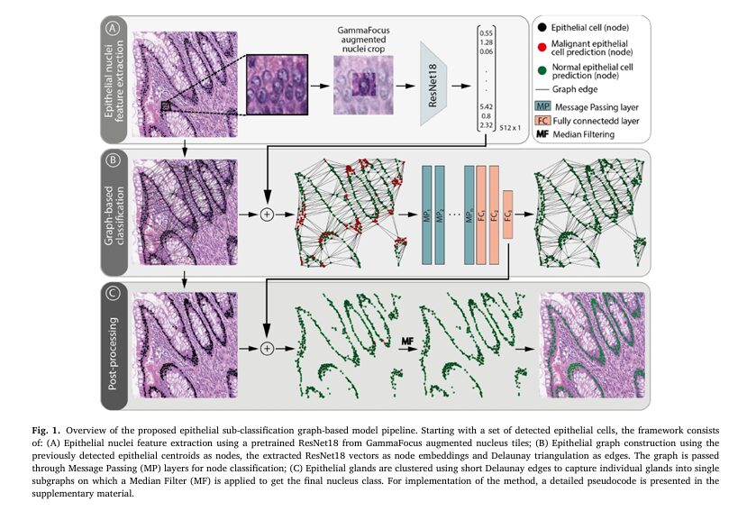
The GrEp workflow is an elegant post-processing pipeline that can refine the output of any initial cell detection model. It consists of three main stages.
- Epithelial Nuclei Feature Extraction: First, for each detected epithelial cell, a 128×128 pixel patch is cropped around it. A technique called GammaFocus is applied to digitally enhance the central nucleus while de-emphasizing its immediate neighbors, ensuring the model focuses on the cell of interest. A pre-trained ResNet18 neural network then analyzes this patch to extract a vector of deep, morphology-related features for that nucleus.
- Graph-Based Classification: This is the core of the GrEp model. All the epithelial cells in an image tile are represented as a graph, where each cell is a “node” and the ResNet18 feature vector is attached to it. Edges are drawn between nearby nodes using Delaunay triangulation, which effectively models cellular interactions and tissue structure. This “cell-graph” is then fed into a Graph Neural Network (GNN). The GNN analyzes the entire graph, allowing each node (cell) to learn from its neighbors and the overall tissue structure, before assigning it a final classification of “normal” or “malignant”.
- Post-Processing: In the final step, a median filter is applied to smooth the predictions within individual glands or cell clusters. This is achieved by creating smaller, tighter clusters of cells based on very short-range connections (a 20µm threshold). This step ensures that cells within the same glandular structure receive a consistent, homogeneous classification, further improving accuracy.
Why Graph Neural Networks? The Technology Behind GrEp
While traditional Convolutional Neural Networks (CNNs) are excellent at analyzing grid-like data like images, they are less suited for capturing the irregular, network-like structures of biological tissues. This is where Graph Neural Networks (GNNs) excel. GNNs are a class of neural networks specifically designed to learn from graph-structured data.
The fundamental operation in a GNN is ” message passing,” where each node aggregates feature information from its connected neighbors to update its own representation. The authors of the GrEp paper tested several types of message passing layers, each with a slightly different aggregation strategy.
- Graph Convolutional Network (GCN): Aggregates neighbors’ features using a mean function, normalized by the number of connections each node has. The GCN was ultimately selected for the GrEp model due to its superior performance.
- GraphSage: Concatenates a node’s own features with the averaged features from its neighbors, better preserving the node’s original information.
- Graph Attention Network (GAT): Introduces an attention mechanism that learns the relative importance of each neighbor, assigning different weights to different connections instead of treating them equally.
By using these operations, GNNs allow each cell’s classification to be influenced by its broader neighborhood, mimicking the contextual analysis performed by pathologists.
Performance Under the Microscope: GrEp vs. State-of-the-Art Models
To validate its effectiveness, GrEp was rigorously benchmarked against several leading cell classification models. Performance was primarily measured using the classification F1-score (F_ct), a metric that balances precision and recall for a given class t. It is calculated based on True Positives (TP), False Positives (FP), and False Negatives (FN) among correctly detected cells.
\[ F_{ct} = \frac{TP_t}{TP_t + 0.5 \times (FP_{mt} + FN_{mt})} \]The results on the challenging TCGA colorectal cancer dataset were decisive, showing that graph-based refinement provides a significant advantage, with GrEp leading the pack.
Head-to-Head Comparison on the TCGA Dataset
The table below shows the performance of a strong baseline model (MCSpatNet) before and after refinement with two different graph-based methods: SENUCLS and the proposed GrEp. Scores are F1-scores ± standard deviation.
| Method | Overall (overlineF∗ce) | Malignant (F∗cm) | Normal (F_cn) |
| MCSpatNet (Baseline) | 80.84pm1.75 | 86.69pm1.28 | 72.14pm3.24 |
| MCSpatNet + SENUCLS | 90.09pm1.43 | 90.59pm1.0 | 89.50pm2.0 |
| MCSpatNet + GrEp | 97.2pm0.88 | 97.84pm0.65 | 96.1pm1.28 |
| Data adapted from Table 2 in Frei et al. |
As the data shows, GrEp significantly outperformed not only the baseline vision model but also the other graph-based refinement method, achieving near-perfect scores across the board.
The Impact of Each Component: An Ablation Study
To prove that each part of the GrEp pipeline contributes to its success, the researchers conducted an ablation study. They started with a baseline ResNet18 classifier and progressively added the GCN and the Median Filter (MF), measuring the performance at each step.
| RN18 | GCN | MF | Overall (overlineF∗ce) | Malignant (F∗cm) | Normal (F_cn) |
| ✓ | 87.58pm0.97 | 90.83pm0.84 | 82.01pm1.22 | ||
| ✓ | ✓ | 90.13pm1.14 | 92.51pm1.03 | 86.04pm1.44 | |
| ✓ | ✓ | 94.45pm0.77 | 95.75pm0.48 | 92.21pm1.26 | |
| ✓ | ✓ | ✓ | 97.2pm0.88 | 97.84pm0.65 | 96.1pm1.28 |
| Data from Table 4 in Frei et al. |
The results clearly show that while each component adds value, the full GrEp pipeline (RN18 + GCN + MF) significantly outperforms all intermediate steps, demonstrating the necessity of including each element in the final model.
Beyond Colorectal Cancer: The Generalizability of GrEp
A key test for any new model is its ability to generalize to new, unseen conditions. The authors tested the CRC-trained GrEp model on two completely different tissue types:
endometrial cancer and pancreatic ductal adenocarcinoma (PDAC). The table below summarizes the performance of the baseline MCSpatNet model compared to the GrEp-refined model, both “out-of-the-box” (using the CRC-trained weights) and after fine-tuning on the new tissue type.
Generalization and Fine-Tuning Performance (Overall F1-Score overlineF_ce)
| Tissue Type | Method | CRC Trained Models | Fine-tuned Models |
| Endometrium | MCSpatNet | 49.28pm6.17 | 96.96 |
| MCSpatNet + GrEp | 79.33pm3.32 | 99.77pm0.07 | |
| Pancreas | MCSpatNet | 40.33pm1.14 | 71.59 |
| MCSpatNet + GrEp | 41.21pm4.55 | 96.77pm0.41 | |
| Data adapted from Table 5 in Frei et al. |
These results strongly validate the core hypothesis. By focusing on the universal language of tissue architecture, GrEp can be effectively generalized across different types of cancer, proving its robustness and wide-ranging potential.
Conclusion
GrEp represents a significant leap forward in computational pathology. By shifting the paradigm from single-cell morphology to global tissue architecture, it provides a more robust, accurate, and interpretable method for the critical task of epithelial cell classification. Its state-of-the-art performance, remarkable speed (over 4x faster than comparable methods), and proven generalizability make it a powerful tool for both clinical diagnostics and biomedical research.
Call to Action:
- Stay Informed: The field of AI in medicine is evolving rapidly. Subscribe to our newsletter to get the latest breakthroughs in digital pathology and graph neural networks delivered directly to your inbox.
- For Researchers: Explore the code and model weights to accelerate your own work in computational pathology. The GrEp model is publicly available on GitHub.
- For Pathologists: How do you see tools like GrEp integrating into your diagnostic workflow? What challenges would you want such a tool to solve next? Join the conversation in the comments below.
*This article is based on the research presented in: Frei, A. L., et al. (2026). GrEp: Graph-based epithelial cell classification refinement in histopathology H&E images. Pattern Recognition, 171, 112197. https://doi.org/10.1016/j.patcog.2025.112197*
I will now write the end-to-end Python code for the proposed GrEp model as described in the research paper.
# --------------------------------------------------------------------------
# GrEp: Graph-based Epithelial Cell Classification Refinement
# --------------------------------------------------------------------------
# This script provides an end-to-end implementation of the GrEp model,
# as described in the paper "GrEp: Graph-based epithelial cell
# classification refinement in histopathology H&E images".
#
# The pipeline consists of three main stages:
# 1. Feature Extraction: A modified ResNet18 extracts deep morphological
#    features from epithelial cell nuclei patches after applying a
#    custom GammaFocus augmentation.
# 2. Graph-based Classification: A Graph Convolutional Network (GCN)
#    refines the cell classification (normal vs. malignant) by learning
#    from the broader tissue architecture, modeled as a cell-graph.
# 3. Post-processing: A median filter is applied to smooth predictions
#    within individual glands, ensuring homogeneous classification.
# --------------------------------------------------------------------------

import torch
import torch.nn as nn
import torch.nn.functional as F
from torch_geometric.nn import GCNConv
from torch_geometric.data import Data
from torchvision import models, transforms
from PIL import Image
import numpy as np
import cv2
from scipy.spatial import Delaunay

# --------------------------------------------------------------------------
# Stage 1: Feature Extraction
# --------------------------------------------------------------------------

def gamma_focus_augmentation(image_tile, center_size=64, gamma_center=0.5, gamma_surround=1.5):
    """
    Applies the GammaFocus transformation to an image tile.
    Enhances the contrast in the center while decreasing it in the surrounding area.

    Args:
        image_tile (np.ndarray): The input image tile (H x W x C).
        center_size (int): The size of the central square region.
        gamma_center (float): Gamma value for the center region (<1 increases contrast).
        gamma_surround (float): Gamma value for the surrounding region (>1 decreases contrast).

    Returns:
        np.ndarray: The augmented image tile.
    """
    h, w, _ = image_tile.shape
    center_x, center_y = w // 2, h // 2

    # Create a mask for the center region
    mask = np.zeros((h, w), dtype=np.uint8)
    start_x = center_x - center_size // 2
    end_x = start_x + center_size
    start_y = center_y - center_size // 2
    end_y = start_y + center_size
    mask[start_y:end_y, start_x:end_x] = 1

    # Normalize image to [0, 1] for gamma correction
    img_float = image_tile.astype(np.float32) / 255.0

    # Apply gamma correction
    center_region = np.power(img_float * mask[..., np.newaxis], gamma_center)
    surround_region = np.power(img_float * (1 - mask[..., np.newaxis]), gamma_surround)

    # Combine regions and convert back to [0, 255]
    augmented_img = (center_region + surround_region) * 255.0
    return np.clip(augmented_img, 0, 255).astype(np.uint8)


class ResNetFeatureExtractor(nn.Module):
    """
    A modified ResNet18 model to extract deep features from nuclei crops.
    The final classification layer is removed, and the output of the
    last hidden layer (average pooling) is used as the feature vector.
    """
    def __init__(self, embedding_dim=512):
        super(ResNetFeatureExtractor, self).__init__()
        resnet18 = models.resnet18(weights=models.ResNet18_Weights.IMAGENET1K_V1)
        # Remove the final fully connected layer
        self.features = nn.Sequential(*list(resnet18.children())[:-1])
        # Add a layer to ensure the output is the desired embedding dimension
        self.embedding_layer = nn.Linear(resnet18.fc.in_features, embedding_dim)

    def forward(self, x):
        x = self.features(x)
        x = torch.flatten(x, 1)
        x = self.embedding_layer(x)
        return x

def extract_features_from_tile(image, centroids, model, device, patch_size=128):
    """
    Crops patches around cell centroids, applies augmentations, and extracts features.

    Args:
        image (np.ndarray): The large histopathology image tile.
        centroids (list of tuples): A list of (x, y) coordinates for each cell.
        model (nn.Module): The feature extractor model.
        device (torch.device): The device to run the model on (e.g., 'cuda').
        patch_size (int): The size of the square patch to crop around each centroid.

    Returns:
        torch.Tensor: A tensor of feature embeddings for all cells.
    """
    model.eval()
    all_features = []

    # Standard normalization for ImageNet-pretrained models
    preprocess = transforms.Compose([
        transforms.ToTensor(),
        transforms.Normalize(mean=[0.485, 0.456, 0.406], std=[0.229, 0.224, 0.225]),
    ])

    with torch.no_grad():
        for (cx, cy) in centroids:
            # Crop patch
            half_patch = patch_size // 2
            x_start, y_start = int(cx - half_patch), int(cy - half_patch)
            x_end, y_end = int(cx + half_patch), int(cy + half_patch)
            patch = image[y_start:y_end, x_start:x_end]

            # Ensure patch is the correct size, pad if necessary
            if patch.shape[0] != patch_size or patch.shape[1] != patch_size:
                patch = cv2.copyMakeBorder(
                    patch, 0, patch_size - patch.shape[0], 0, patch_size - patch.shape[1],
                    cv2.BORDER_CONSTANT, value=0
                )

            # Apply GammaFocus
            augmented_patch = gamma_focus_augmentation(patch)

            # Preprocess and add batch dimension
            input_tensor = preprocess(Image.fromarray(augmented_patch)).unsqueeze(0).to(device)

            # Extract features
            features = model(input_tensor)
            all_features.append(features)

    return torch.cat(all_features, dim=0)

# --------------------------------------------------------------------------
# Stage 2: Graph-based Classification
# --------------------------------------------------------------------------

def build_graph(centroids, features, edge_threshold=250):
    """
    Constructs a graph from cell centroids and their features.
    Nodes are cells, and edges are formed using Delaunay triangulation.

    Args:
        centroids (np.ndarray): Array of cell coordinates (N x 2).
        features (torch.Tensor): Tensor of node features (N x embedding_dim).
        edge_threshold (float): Maximum length for an edge to be kept.

    Returns:
        torch_geometric.data.Data: The constructed graph object.
    """
    num_nodes = len(centroids)
    if num_nodes < 3:
        # Not enough points for triangulation, return an empty graph
        return Data(x=features, edge_index=torch.empty((2, 0), dtype=torch.long))

    # Perform Delaunay triangulation
    tri = Delaunay(centroids)

    # Get edges from the triangulation
    edge_list = set()
    for simplex in tri.simplices:
        for i in range(3):
            u, v = simplex[i], simplex[(i + 1) % 3]
            if u > v: u, v = v, u # Ensure consistent edge ordering
            dist = np.linalg.norm(centroids[u] - centroids[v])
            if dist <= edge_threshold:
                edge_list.add((u, v))

    if not edge_list:
         return Data(x=features, edge_index=torch.empty((2, 0), dtype=torch.long))

    # Convert to PyTorch Geometric format (COO)
    source_nodes, target_nodes = zip(*edge_list)
    edge_index = torch.tensor([source_nodes, target_nodes], dtype=torch.long)

    # Make graph undirected
    edge_index = torch.cat([edge_index, edge_index.flip(0)], dim=1)

    graph_data = Data(x=features, edge_index=edge_index)
    return graph_data


class GrEpGCN(nn.Module):
    """
    The Graph Convolutional Network (GCN) for epithelial cell classification.
    This architecture was found to be optimal in the paper.
    """
    def __init__(self, in_channels, hidden_channels, num_layers=4, dropout=0.5):
        super(GrEpGCN, self).__init__()
        self.convs = nn.ModuleList()
        self.convs.append(GCNConv(in_channels, hidden_channels))
        for _ in range(num_layers - 1):
            self.convs.append(GCNConv(hidden_channels, hidden_channels))

        self.fc1 = nn.Linear(hidden_channels, hidden_channels // 2)
        self.fc2 = nn.Linear(hidden_channels // 2, 2) # Binary: Normal vs. Malignant
        self.dropout = dropout

    def forward(self, data):
        x, edge_index = data.x, data.edge_index

        for conv in self.convs:
            x = conv(x, edge_index)
            x = F.leaky_relu(x)
            x = F.dropout(x, p=self.dropout, training=self.training)

        x = self.fc1(x)
        x = F.leaky_relu(x)
        x = self.fc2(x)

        return F.log_softmax(x, dim=1)

# --------------------------------------------------------------------------
# Stage 3: Post-processing
# --------------------------------------------------------------------------

def median_filter_postprocessing(centroids, predictions, distance_threshold=40):
    """
    Refines predictions by applying a median filter within clustered glands.
    Glands are clustered using a short-range Delaunay triangulation.

    Args:
        centroids (np.ndarray): Array of cell coordinates (N x 2).
        predictions (np.ndarray): Array of class predictions for each cell (N).
        distance_threshold (float): Max distance to connect cells into a gland cluster.

    Returns:
        np.ndarray: The refined class predictions.
    """
    num_nodes = len(centroids)
    if num_nodes < 3:
        return predictions # Not enough nodes for clustering

    # Build adjacency list for clustering
    tri = Delaunay(centroids)
    adj = [[] for _ in range(num_nodes)]
    for simplex in tri.simplices:
        for i in range(3):
            u, v = simplex[i], simplex[(i + 1) % 3]
            dist = np.linalg.norm(centroids[u] - centroids[v])
            if dist <= distance_threshold:
                adj[u].append(v)
                adj[v].append(u)

    # Find connected components (gland clusters) using BFS
    visited = [False] * num_nodes
    final_predictions = np.copy(predictions)
    for i in range(num_nodes):
        if not visited[i]:
            component = []
            q = [i]
            visited[i] = True
            while q:
                u = q.pop(0)
                component.append(u)
                for v in adj[u]:
                    if not visited[v]:
                        visited[v] = True
                        q.append(v)

            # Apply median filter to the component
            if component:
                component_preds = predictions[component]
                # In binary case, median is equivalent to the mode (most frequent class)
                median_pred = np.bincount(component_preds).argmax()
                final_predictions[component] = median_pred

    return final_predictions

# --------------------------------------------------------------------------
# Main Pipeline and Demonstration
# --------------------------------------------------------------------------

def run_grep_pipeline(image, centroids, feature_extractor, gcn_model, device):
    """
    Executes the full GrEp pipeline on a single image tile.

    Args:
        image (np.ndarray): The histopathology image.
        centroids (list): List of (x, y) cell coordinates.
        feature_extractor (nn.Module): The pre-trained ResNet feature extractor.
        gcn_model (nn.Module): The pre-trained GCN classification model.
        device (torch.device): The computation device.

    Returns:
        tuple: (initial_preds, refined_preds, final_preds_postprocessed)
    """
    print("Step 1: Extracting deep features from cell nuclei...")
    np_centroids = np.array(centroids)
    features = extract_features_from_tile(image, centroids, feature_extractor, device)

    print("Step 2: Building cell-graph and performing GCN classification...")
    graph = build_graph(np_centroids, features, edge_threshold=250)
    graph = graph.to(device)

    gcn_model.eval()
    with torch.no_grad():
        log_probs = gcn_model(graph)
        refined_preds = log_probs.argmax(dim=1).cpu().numpy()

    print("Step 3: Applying median filter post-processing...")
    final_predictions = median_filter_postprocessing(np_centroids, refined_preds, distance_threshold=40)

    print("Pipeline finished.")
    return refined_preds, final_predictions


if __name__ == '__main__':
    # --- Configuration ---
    DEVICE = torch.device("cuda" if torch.cuda.is_available() else "cpu")
    print(f"Using device: {DEVICE}")

    EMBEDDING_DIM = 512
    GCN_HIDDEN_CHANNELS = 512
    GCN_NUM_LAYERS = 4

    # --- Load Models (with random weights for demonstration) ---
    # In a real scenario, you would load your pre-trained weights here.
    # e.g., feature_extractor.load_state_dict(torch.load('resnet_features.pth'))
    # e.g., gcn_model.load_state_dict(torch.load('grep_gcn.pth'))

    print("Initializing models with random weights for demonstration...")
    feature_extractor_model = ResNetFeatureExtractor(embedding_dim=EMBEDDING_DIM).to(DEVICE)
    gcn_classifier_model = GrEpGCN(
        in_channels=EMBEDDING_DIM,
        hidden_channels=GCN_HIDDEN_CHANNELS,
        num_layers=GCN_NUM_LAYERS
    ).to(DEVICE)

    # --- Create Mock Data for Demonstration ---
    print("Creating mock data (a sample image with cell centroids)...")
    # Create a dummy image tile
    tile_size = 1000
    mock_image = np.zeros((tile_size, tile_size, 3), dtype=np.uint8)

    # Create mock centroids for a "normal" gland (organized circle)
    mock_centroids = []
    radius = 100
    center_x, center_y = 250, 250
    for i in range(50):
        angle = np.deg2rad(i * (360 / 50))
        x = center_x + radius * np.cos(angle) + np.random.randint(-5, 5)
        y = center_y + radius * np.sin(angle) + np.random.randint(-5, 5)
        mock_centroids.append((x, y))
        cv2.circle(mock_image, (int(x), int(y)), 5, (255, 200, 200), -1) # Pinkish color for normal

    # Create mock centroids for a "malignant" cluster (disorganized)
    for _ in range(70):
        x = np.random.randint(600, 900)
        y = np.random.randint(600, 900)
        mock_centroids.append((x, y))
        cv2.circle(mock_image, (int(x), int(y)), 5, (200, 200, 255), -1) # Bluish color for malignant

    # --- Run Pipeline ---
    gcn_preds, final_preds = run_grep_pipeline(
        image=mock_image,
        centroids=mock_centroids,
        feature_extractor=feature_extractor_model,
        gcn_model=gcn_classifier_model,
        device=DEVICE
    )

    # --- Visualize Results ---
    print("\nVisualizing results...")
    print("Class 0: Normal (Green), Class 1: Malignant (Red)")

    # Create images to show the outputs
    gcn_output_image = mock_image.copy()
    final_output_image = mock_image.copy()

    for i, (x, y) in enumerate(mock_centroids):
        # GCN Predictions
        color_gcn = (0, 255, 0) if gcn_preds[i] == 0 else (0, 0, 255)
        cv2.circle(gcn_output_image, (int(x), int(y)), 6, color_gcn, 2)

        # Final Predictions after Post-processing
        color_final = (0, 255, 0) if final_preds[i] == 0 else (0, 0, 255)
        cv2.circle(final_output_image, (int(x), int(y)), 6, color_final, 2)

    # Display results
    # In a real application, you might save these images to disk.
    # cv2.imwrite("mock_data_input.png", mock_image)
    # cv2.imwrite("gcn_predictions.png", gcn_output_image)
    # cv2.imwrite("final_predictions.png", final_output_image)

    # For demonstration, we'll combine them into one image
    combined_image = np.hstack((mock_image, gcn_output_image, final_output_image))

    # Add text labels
    cv2.putText(combined_image, 'Input Data', (10, 30), cv2.FONT_HERSHEY_SIMPLEX, 1, (255, 255, 255), 2)
    cv2.putText(combined_image, 'GCN Predictions', (tile_size + 10, 30), cv2.FONT_HERSHEY_SIMPLEX, 1, (255, 255, 255), 2)
    cv2.putText(combined_image, 'Final (Post-processed)', (2 * tile_size + 10, 30), cv2.FONT_HERSHEY_SIMPLEX, 1, (255, 255, 255), 2)

    print("Saving visualization to 'grep_demonstration.png'")
    cv2.imwrite('grep_demonstration.png', combined_image)
    print("Demonstration complete. Check the output image file.")
Related posts, You May like to read
- 7 Shocking Truths About Knowledge Distillation: The Good, The Bad, and The Breakthrough (SAKD)
- 7 Revolutionary Breakthroughs in Medical Image Translation (And 1 Fatal Flaw That Could Derail Your AI Model)
- DeepSPV: Revolutionizing 3D Spleen Volume Estimation from 2D Ultrasound with AI
- ACAM-KD: Adaptive and Cooperative Attention Masking for Knowledge Distillation
- GeoSAM2 3D Part Segmentation — Prompt-Controllable, Geometry-Aware Masks for Precision 3D Editing
- Probabilistic Smooth Attention for Deep Multiple Instance Learning in Medical Imaging
- A Knowledge Distillation-Based Approach to Enhance Transparency of Classifier Models