As the world transitions toward clean and sustainable energy, power systems are increasingly integrating renewable energy resources (RERs) such as solar photovoltaic (PV) and wind power. While these sources reduce carbon emissions and operational costs, their inherent uncertainty and intermittency pose significant challenges to maintaining grid stability and efficiency. One of the most critical tools for managing modern power networks is the Optimal Power Flow (OPF) problem, which determines the optimal operating state of a power system while minimizing costs and satisfying technical constraints.
However, traditional OPF methods struggle when applied to systems with high RER penetration due to unpredictable generation patterns. To address this, researchers have developed advanced optimization techniques—among them, the Improved Pelican Optimization Algorithm (IPOA)—a novel metaheuristic approach designed specifically for stochastic OPF (S-OPF) problems under uncertainty.
In this article, we explore how IPOA enhances the performance of the original Pelican Optimization Algorithm (POA), its application in solving S-OPF with solar and wind integration, and why it outperforms other state-of-the-art algorithms in both accuracy and convergence speed.
What Is Stochastic Optimal Power Flow?
The Optimal Power Flow (OPF) problem aims to minimize an objective function—such as fuel cost or emissions—while ensuring that all physical and operational constraints of the power system are satisfied. These include:
- Active and reactive power balance
- Voltage limits at buses
- Generator output bounds
- Transformer tap settings
- Transmission line capacity
When renewable energy sources like wind and solar are introduced, their variable nature introduces stochasticity, making deterministic OPF insufficient. This leads to the Stochastic Optimal Power Flow (S-OPF) framework, which accounts for uncertainties in wind speed, solar irradiance, and load demand using probabilistic models.
Why Traditional Methods Fall Short
Conventional optimization techniques like Newton-Raphson, gradient-based, or interior-point methods often suffer from:
- Slow convergence
- Getting trapped in local optima
- Inability to handle non-convex, non-linear, and multi-modal functions
To overcome these limitations, metaheuristic algorithms inspired by nature—such as Genetic Algorithms, Particle Swarm Optimization (PSO), and Grey Wolf Optimizer (GWO)—have gained popularity. However, even these can stagnate or lack sufficient exploration-exploitation balance.
That’s where the Improved Pelican Optimization Algorithm (IPOA) comes into play.
The Pelican Optimization Algorithm: Nature-Inspired Intelligence
Introduced in 2022, the Pelican Optimization Algorithm (POA) mimics the hunting behavior of pelicans, particularly their two-phase strategy:
- Exploration Phase: Pelicans scan large areas to locate prey.
- Exploitation Phase: Once near the target, they dive and use wing movements to herd fish into their pouches.
While POA shows promise, it suffers from premature convergence and limited search diversity, especially in complex, high-dimensional problems like S-OPF.
To enhance its performance, the authors of the study proposed three key improvements, forming the Improved Pelican Optimization Algorithm (IPOA).
Key Innovations in the Improved Pelican Optimization Algorithm (IPOA)
The IPOA integrates three novel strategies to boost exploration, avoid local optima, and accelerate convergence:
1. Mutation-Based Strategy
This mechanism introduces genetic variation into the population using two mutation operators:
- Conservative Mutation:
- Current-to-Best Mutation:
Here, F is a scaling factor, and indices m1,m2,m3,m4 are randomly selected individuals different from i . This diversifies the search space and prevents premature convergence.
2. Fitness Distance Balanced (FDB) Selection
The FDB strategy improves selection pressure by balancing fitness value and distance from the best solution. It calculates a score for each individual based on normalized fitness and spatial distance:
\[ DS_i = \sum_{j=1}^{d} \big(x_{i,j} – Best_j \big)^{2} \]Normalized values:
\[ \text{normDS}_i = \frac{DS_i – \min(DS)}{\max(DS) – \min(DS)}, \qquad \text{normF}_i = \frac{F_i – \min(F)}{\max(F) – \min(F)} \]Final FDB score:
\[ \text{FDBscore}_i = \alpha \cdot \big(1 – \text{norm}F_i\big) + (1 – \alpha) \cdot \text{norm}DS_i \]
where α = 0.5⋅(1+ t / Tmax) increases exploitation over time.
This ensures a balanced transition from global exploration to local refinement.
3. Exploitation-Based Gorilla Troops Optimizer (GTO)
Inspired by gorilla social dynamics, the GTO component simulates how silverback leaders guide troop movement. The update equation is:
\[ GX(t+1) = L \cdot M \cdot \big( X(t) – X_{\text{silverback}} \big) + X(t) \]where:
\[ M = \left( \frac{\sum_{i=1}^{N} X_i(t)}{2L} \right)^{\frac{1}{2L}} \] \[ L = C \cdot l, \quad C = \big(\cos(2r^5) + 1\big)\cdot\left(1 – \frac{t}{T_{\max}}\right) \] \[ l \in [-1, 1] \quad \text{is random} \]This enhances local search capability and fine-tunes solutions during later iterations.
✅ Together, these enhancements make IPOA more robust, accurate, and adaptable to complex engineering problems like S-OPF.
Modeling Uncertainty in Wind and Solar Generation
For S-OPF to be effective, realistic models of RER uncertainty must be incorporated.
Wind Power Uncertainty
Wind speed follows a Weibull probability density function (PDF):
\[ f_v(v) = (c k)\,(c v)^{k-1} e^{-(c v)^k}, \quad v > 0 \]Where:
- k : shape parameter
- c : scale parameter
- Mean wind speed: Mwbl = c⋅Γ (1+k−1)
Wind turbine output depends on cut-in (vin ), rated (vr ), and cut-out (vout ) speeds:
\[ P_w(v) = \begin{cases} 0, & v < v_{\text{in}} \ \text{or} \ v > v_{\text{out}} \\[6pt] \dfrac{P_w \cdot v_r}{v_r – v_{\text{in}}}(v – v_{\text{in}}), & v_{\text{in}} \leq v \leq v_r \\[10pt] P_w, & v_r < v \leq v_{\text{out}} \end{cases} \]
Assumed values: vin = 3 , vr = 16 , vout = 25 m/s.
Solar PV Uncertainty
Solar irradiance is modeled using a lognormal PDF:
\[ f_I(I) = \frac{1}{I \sigma \sqrt{2\pi}} \exp\!\left(-\frac{(\ln I – \mu)^2}{2\sigma^2}\right), \quad I > 0 \]PV output:
\[ P_{pv}(I) = \begin{cases} \dfrac{P_{pvr} \cdot I_{std}}{I}, & I \geq I_c \\[8pt] \dfrac{P_{pvr} \cdot I_{std} \cdot I_c}{I^2}, & 0 < I < I_c \end{cases} \]
Where Ic is the threshold irradiance and Istd is standard test condition irradiance.
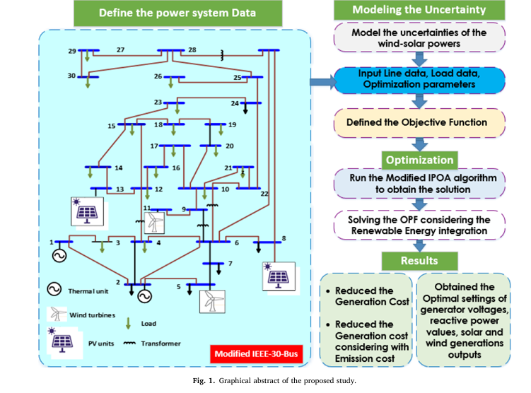
These models were integrated into a modified IEEE 30-bus system with wind farms at buses 5 and 11 (75 MW and 60 MW), and solar PV units also connected at those locations.
Objective Functions: Minimizing Cost and Emissions
The S-OPF problem considers two main objectives.
Objective 1: Total Generation Cost Minimization
Includes thermal, wind, and solar costs, including penalties for over/underestimation.
Thermal Fuel Cost (with valve-point effect):
\[ \varsigma_T(P^{TG}) = \sum_{i=1}^{N_{tg}} \Big( a_i P_{gi}^2 + b_i P_{gi} + c_i + \big| d_i \sin\big(e_i (P_{Gi}^{\min} – P_{Gi})\big) \big| \Big) \]Wind and Solar Direct Costs:
\[ \lambda_{ws,j}(P_{ws,j}) = g_j \, P_{ws,j}, \qquad \lambda_{pvs,k}(P_{pvs,k}) = h_k \, P_{pvs,k} \]
Reserve and Penalty Costs:
For wind:
\[ \xi_{w,j}(P_{w,j}) = \lambda_{ws,j} + \lambda_{wr,j}\big(P_{ws,j} – P_{wav,j}\big) + \lambda_{wp,j}\big(P_{wav,j} – P_{ws,j}\big) \]For solar:
\[ \xi_{pv,k}(P_{pv,k}) = \lambda_{pvs,k} \;+\; \lambda_{pvr,k}\,(P_{pvs,k} – P_{pva,k}) \;+\; \lambda_{pvp,k}\,(P_{pva,k} – P_{pvs,k}) \]Full Objective Function:
\[ F_{1} = \varsigma T(P_{TG}) \;+\; \sum_{j} \xi_{w,j} \;+\; \sum_{k} \xi_{pv,k} \]
Objective 2: Emission-Aware Cost Minimization
Carbon emissions from thermal units:
\[ E = \sum_{i=1}^{N_{TG}} \Big[ (\alpha_i + \beta_i P_{TG,i} + \gamma_i P_{TG,i}^2)\times 0.01 \;+\; \omega_i \cdot e^{\mu_i P_{TG,i}} \Big] \] \[\text{With carbon tax} ( C_{\text{tax}} = $20/\text{ton} )\]: \[ F_2 = F_1 + C_{\text{tax}} \cdot E \]Performance Evaluation: IPOA vs. State-of-the-Art Algorithms
The IPOA was tested against five powerful optimizers:
- Sand Cat Swarm Optimization (SCSO)
- Grey Wolf Optimizer (GWO)
- Zebra Optimization Algorithm (ZOA)
- Dandelion Optimizer (DO)
- Original Pelican Optimization Algorithm (POA)
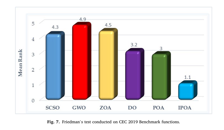
Benchmark Testing: CEC 2019 Functions
| FUNCTION | BEST SOLVER | IPOA RANK |
|---|---|---|
| G1 | IPOA | 1st |
| G2 | IPOA | 1st |
| G3 | Tie | Top |
| G4 | DO | 2nd |
| G5 | IPOA | 1st |
| G6 | DO (best), IPOA (mean) | 1st (avg) |
| G7 | IPOA | 1st |
| G8–G10 | IPOA | 1st |
Statistical tests confirmed significant superiority:
- Wilcoxon rank-sum test: p-values < 0.05 for most cases
- Friedman test: IPOA ranked first overall
Case Studies: Application to Modified IEEE 30-Bus System
Two scenarios were evaluated:
Case 1: Generation Cost Reduction (No Emissions)
| ALGORITHM | BEST COST ($) | AVG.COST) | STD DEV |
|---|---|---|---|
| SCSO | 862.00 | 862.60 | 0.36 |
| GWO | 862.06 | 862.46 | 0.25 |
| DO | 861.92 | 862.29 | 0.26 |
| IPOA | 861.89 | 861.93 | 0.06 |
✅ IPOA achieved the lowest cost and highest stability.
Case 2: Emission-Constrained Cost Minimization
| ALGORITHM | BEST COST ($) | AVG. COST ($) | STD DEV |
|---|---|---|---|
| DO | 892.1585 | 892.2261 | 0.122 |
| IPOA | 892.1538 | 892.1803 | 0.120 |
Despite tighter constraints, IPOA delivered the best solution, reducing emissions to 0.885 ton/h and power losses to 5.4486 MW.
📈 Convergence plots show IPOA reaches optimal solutions faster than competitors, often within 30–40 iterations.
🏆 Why IPOA Outperforms Other Algorithms
| FEATURES | IPOA ADVANTAGES |
|---|---|
| Exploration | Mutation + FDB ensures diverse initial search |
| Exploitation | GTO-based refinement improves local search |
| Balance | Dynamic α in FDB balances exploration/exploitation |
| Robustness | Handles non-convex, noisy, multi-modal landscapes |
| Speed | Faster convergence due to guided updates |
Moreover, IPOA maintains all system variables within feasible limits (voltage, reactive power, transformer taps), proving its practical applicability.
🔮 Future Applications and Research Directions
The success of IPOA opens doors for:
- Large-scale grid integration with multiple RERs
- Electric vehicle (EV) charging coordination
- Microgrid energy management
- Real-time dispatch in smart grids
Future work may involve hybridizing IPOA with machine learning models for predictive optimization or applying it to multi-objective OPF with environmental and economic trade-offs.
✅ Conclusion: A Leap Forward in Power System Optimization
The Improved Pelican Optimization Algorithm (IPOA) represents a major advancement in solving stochastic optimal power flow problems in modern power systems. By integrating mutation strategies, fitness-distance balance, and gorilla troops exploitation, IPOA achieves superior performance in terms of:
- Solution quality
- Convergence speed
- Stability
- Constraint handling
Validated through rigorous testing on CEC 2019 benchmarks and real-world IEEE 30-bus case studies, IPOA consistently outperforms leading metaheuristics like GWO, DO, and POA in minimizing generation costs and emissions under renewable uncertainty.
As power systems grow more complex and decentralized, intelligent algorithms like IPOA will become essential tools for engineers, planners, and policymakers striving for affordable, reliable, and sustainable electricity.
Call to Action: Join the Energy Optimization Revolution!
Are you working on power system optimization, renewable integration, or smart grid technologies? Download the full research paper to dive deeper into the IPOA methodology, equations, and simulation data.
👉 Click here to access the complete study
💡 Want to implement IPOA in your project?
Contact the corresponding authors:
- Hamed Zeinoddini-Meymand: h.zeinaddini@gmail.com
- Farhad Shahnia: F.Shahnia@murdoch.edu.au
🔗 Follow us for more insights on AI-driven energy solutions, optimization algorithms, and sustainable grid technologies.
Let’s build a smarter, cleaner energy future—together.
I’ll provide a complete Python implementation of the Improved Pelican Optimization Algorithm (IPOA) for solving the stochastic optimal power flow problem as described in the paper. This implementation includes the uncertainty modeling of renewable energy resources and the three improvement strategies.
import numpy as np
import matplotlib.pyplot as plt
from scipy.stats import weibull_min, lognorm
from scipy.special import gamma
import pandas as pd
import time

class IPOA:
    def __init__(self, n_pop, n_iter, problem_dim, lb, ub, objective_func):
        self.n_pop = n_pop
        self.n_iter = n_iter
        self.problem_dim = problem_dim
        self.lb = lb
        self.ub = ub
        self.objective_func = objective_func

        # Initialize population
        self.population = np.random.uniform(lb, ub, (n_pop, problem_dim))
        self.fitness = np.zeros(n_pop)
        self.best_solution = None
        self.best_fitness = float('inf')
        self.fitness_history = []

        # Parameters for improvements
        self.F = 0.5  # Scaling factor for mutation
        self.a = 0.5  # Initial weight for FDB
        self.betamin = 0.2
        self.betamax = 0.8
        self.p = 0.03
        self.w = 0.8

    def initialize_population(self):
        self.population = np.random.uniform(self.lb, self.ub, (self.n_pop, self.problem_dim))
        for i in range(self.n_pop):
            self.fitness[i] = self.objective_func(self.population[i])

            if self.fitness[i] < self.best_fitness:
                self.best_fitness = self.fitness[i]
                self.best_solution = self.population[i].copy()

        self.fitness_history.append(self.best_fitness)

    def mutation_strategy(self, current_iter):
        mutated_population = np.zeros_like(self.population)

        for i in range(self.n_pop):
            # Select three random individuals
            r1, r2, r3 = np.random.choice(range(self.n_pop), 3, replace=False)

            # Conventional mutation
            if np.random.rand() < 0.5:
                mutated_population[i] = self.population[r1] + self.F * (self.population[r2] - self.population[r3])
            # Current-to-best mutation
            else:
                r4 = np.random.randint(0, self.n_pop)
                mutated_population[i] = self.best_solution + self.F * (self.population[r1] - self.population[r2]) + \
                                       self.F * (self.population[r3] - self.population[r4])

            # Apply bounds
            mutated_population[i] = np.clip(mutated_population[i], self.lb, self.ub)

        return mutated_population

    def FDB_selection(self, current_iter):
        # Calculate distance matrix
        DS = np.zeros(self.n_pop)
        for i in range(self.n_pop):
            DS[i] = np.sqrt(np.sum((self.population[i] - self.best_solution)**2))

        # Normalize distance and fitness
        normDS = (DS - np.min(DS)) / (np.max(DS) - np.min(DS) + 1e-10)
        normF = (self.fitness - np.min(self.fitness)) / (np.max(self.fitness) - np.min(self.fitness) + 1e-10)

        # Update weight parameter
        self.a = 0.5 * (1 + current_iter / self.n_iter)

        # Calculate FDB score
        FDBscore = self.a * (1 - normF) + (1 - self.a) * normDS

        return FDBscore

    def GTO_exploitation(self, current_iter):
        # Calculate M parameter
        M = (np.abs(np.sum(self.population, axis=0) / self.n_pop) ** (2 ** np.random.rand())) ** (1 / (2 ** np.random.rand()))

        # Calculate C parameter
        C = (np.cos(2 * np.random.rand()) + 1) * (1 - current_iter / self.n_iter)

        # Calculate L parameter
        L = C * np.random.uniform(-1, 1, self.problem_dim)

        # Apply GTO mechanism
        GX = L * M * (self.population - self.best_solution) + self.population

        # Apply bounds
        GX = np.clip(GX, self.lb, self.ub)

        return GX

    def optimize(self):
        self.initialize_population()

        for iter in range(self.n_iter):
            # Phase 1: Exploration (moving towards prey)
            new_population_1 = np.zeros_like(self.population)
            for i in range(self.n_pop):
                if self.fitness[i] > self.best_fitness:
                    new_population_1[i] = self.population[i] + np.random.rand() * (self.best_solution - self.population[i])
                else:
                    new_population_1[i] = self.population[i] + np.random.rand() * (self.population[i] - self.best_solution)

            # Apply bounds
            new_population_1 = np.clip(new_population_1, self.lb, self.ub)

            # Evaluate new population
            new_fitness_1 = np.zeros(self.n_pop)
            for i in range(self.n_pop):
                new_fitness_1[i] = self.objective_func(new_population_1[i])

                # Update if better
                if new_fitness_1[i] < self.fitness[i]:
                    self.population[i] = new_population_1[i]
                    self.fitness[i] = new_fitness_1[i]

                    if new_fitness_1[i] < self.best_fitness:
                        self.best_fitness = new_fitness_1[i]
                        self.best_solution = new_population_1[i].copy()

            # Phase 2: Exploitation (whizzing on water surface)
            R = 0.2
            new_population_2 = np.zeros_like(self.population)
            for i in range(self.n_pop):
                new_population_2[i] = self.population[i] + R * (1 - iter/self.n_iter) * (2*np.random.rand() - 1) * self.population[i]

            # Apply bounds
            new_population_2 = np.clip(new_population_2, self.lb, self.ub)

            # Evaluate new population
            new_fitness_2 = np.zeros(self.n_pop)
            for i in range(self.n_pop):
                new_fitness_2[i] = self.objective_func(new_population_2[i])

                # Update if better
                if new_fitness_2[i] < self.fitness[i]:
                    self.population[i] = new_population_2[i]
                    self.fitness[i] = new_fitness_2[i]

                    if new_fitness_2[i] < self.best_fitness:
                        self.best_fitness = new_fitness_2[i]
                        self.best_solution = new_population_2[i].copy()

            # Apply improvement strategies
            # 1. Mutation strategy
            mutated_pop = self.mutation_strategy(iter)
            for i in range(self.n_pop):
                mut_fitness = self.objective_func(mutated_pop[i])
                if mut_fitness < self.fitness[i]:
                    self.population[i] = mutated_pop[i]
                    self.fitness[i] = mut_fitness

                    if mut_fitness < self.best_fitness:
                        self.best_fitness = mut_fitness
                        self.best_solution = mutated_pop[i].copy()

            # 2. FDB selection
            FDBscore = self.FDB_selection(iter)
            # Sort by FDBscore (lower is better)
            sorted_indices = np.argsort(FDBscore)
            self.population = self.population[sorted_indices]
            self.fitness = self.fitness[sorted_indices]

            # 3. GTO exploitation
            GTO_pop = self.GTO_exploitation(iter)
            for i in range(self.n_pop):
                GTO_fitness = self.objective_func(GTO_pop[i])
                if GTO_fitness < self.fitness[i]:
                    self.population[i] = GTO_pop[i]
                    self.fitness[i] = GTO_fitness

                    if GTO_fitness < self.best_fitness:
                        self.best_fitness = GTO_fitness
                        self.best_solution = GTO_pop[i].copy()

            # Record best fitness
            self.fitness_history.append(self.best_fitness)

            # Print progress
            if iter % 10 == 0:
                print(f"Iteration {iter}, Best Fitness: {self.best_fitness}")

        return self.best_solution, self.best_fitness, self.fitness_history

# Stochastic OPF problem formulation
class StochasticOPF:
    def __init__(self):
        # System parameters (based on IEEE 30-bus system)
        self.n_buses = 30
        self.n_gen = 6  # including renewable generators
        self.n_wind = 2
        self.n_solar = 2

        # Cost coefficients for thermal generators
        self.a_i = np.array([0.00375, 0.0175, 0.0625, 0.00834, 0.025, 0.025])
        self.b_i = np.array([2.00, 1.75, 1.00, 3.25, 3.00, 3.00])
        self.c_i = np.array([0, 0, 0, 0, 0, 0])

        # Valve-point loading effect coefficients
        self.d_i = np.array([0.063, 0.098, 0.082, 0.056, 0.052, 0.052])
        self.e_i = np.array([0.041, 0.036, 0.028, 0.024, 0.022, 0.022])

        # Wind cost coefficients
        self.g_i = np.array([1.5, 1.5])  # $/MWh
        self.K_wrj = np.array([3.0, 3.0])  # reserve cost coefficient
        self.K_wpj = np.array([1.5, 1.5])  # penalty cost coefficient

        # Solar cost coefficients
        self.h_k = np.array([1.8, 1.8])  # $/MWh
        self.K_pnrk = np.array([2.5, 2.5])  # reserve cost coefficient
        self.K_ppk = np.array([1.2, 1.2])  # penalty cost coefficient

        # Emission coefficients
        self.alpha_i = np.array([4.091, 2.543, 4.258, 5.326, 4.258, 6.131])
        self.beta_i = np.array([-5.554, -6.047, -5.094, -3.55, -5.094, -5.555])
        self.gamma_i = np.array([6.49, 5.638, 4.586, 3.38, 4.586, 5.151])
        self.eta_i = np.array([2.0e-4, 5.0e-4, 1.0e-6, 2.0e-3, 1.0e-6, 1.0e-5])
        self.delta_i = np.array([2.857, 3.333, 8.000, 2.000, 8.000, 6.667])

        # Carbon tax
        self.C_tax = 20  # $/ton

        # Wind parameters
        self.v_in = 3  # m/s, cut-in speed
        self.v_r = 16  # m/s, rated speed
        self.v_out = 25  # m/s, cut-out speed
        self.P_wr = np.array([75, 60])  # MW, rated power of wind farms

        # Solar parameters
        self.I_c = 120  # W/m², certain irradiance
        self.I_std = 1000  # W/m², standard irradiance
        self.P_prr = np.array([35, 50])  # MW, rated power of solar PV units

        # Weibull parameters for wind (k, c)
        self.wind_params = np.array([[2.0, 8.0], [2.0, 8.0]])

        # Lognormal parameters for solar (mu, sigma)
        self.solar_params = np.array([[5.5, 0.5], [5.5, 0.5]])

        # Power limits
        self.P_min = np.array([50, 20, 15, 10, 10, 12])  # MW
        self.P_max = np.array([140, 80, 50, 35, 30, 40])  # MW
        self.Q_min = np.array([-20, -20, -15, -15, -10, -12])  # MVAR
        self.Q_max = np.array([150, 60, 50, 40, 30, 40])  # MVAR
        self.V_min = 0.95  # p.u.
        self.V_max = 1.1  # p.u.

        # Load data (simplified)
        self.P_load = 283.4  # MW
        self.Q_load = 126.2  # MVAR

        # Number of scenarios for Monte Carlo simulation
        self.n_scenarios = 1000

    def weibull_pdf(self, v, k, c):
        """Weibull probability density function"""
        return (k/c) * (v/c)**(k-1) * np.exp(-(v/c)**k)

    def lognormal_pdf(self, I, mu, sigma):
        """Lognormal probability density function"""
        return (1/(I * sigma * np.sqrt(2*np.pi))) * np.exp(-(np.log(I)-mu)**2/(2*sigma**2))

    def wind_power(self, v):
        """Wind power output as function of wind speed"""
        P_w = np.zeros_like(v)
        for i in range(len(v)):
            if v[i] < self.v_in or v[i] > self.v_out:
                P_w[i] = 0
            elif v[i] < self.v_r:
                P_w[i] = self.P_wr * ((v[i] - self.v_in) / (self.v_r - self.v_in))
            else:
                P_w[i] = self.P_wr
        return P_w

    def solar_power(self, I):
        """Solar power output as function of irradiance"""
        P_p = np.zeros_like(I)
        for i in range(len(I)):
            if I[i] <= 0:
                P_p[i] = 0
            elif I[i] < self.I_c:
                P_p[i] = self.P_prr * (I[i]**2 / (self.I_std * self.I_c))
            else:
                P_p[i] = self.P_prr * (I[i] / self.I_std)
        return P_p

    def thermal_cost(self, P_g):
        """Quadratic fuel cost with valve-point loading effect"""
        cost = 0
        for i in range(len(P_g)):
            cost += self.a_i[i] * P_g[i]**2 + self.b_i[i] * P_g[i] + self.c_i[i] + \
                   self.d_i[i] * np.abs(np.sin(self.e_i[i] * (self.P_min[i] - P_g[i])))
        return cost

    def wind_direct_cost(self, P_ws):
        """Direct cost of scheduled wind power"""
        return np.sum(self.g_i * P_ws)

    def wind_reserve_cost(self, P_ws, P_wav):
        """Reserve cost for wind power"""
        cost = 0
        for j in range(self.n_wind):
            if P_ws[j] > P_wav[j]:
                cost += self.K_wrj[j] * (P_ws[j] - P_wav[j])
        return cost

    def wind_penalty_cost(self, P_ws, P_wav):
        """Penalty cost for wind power"""
        cost = 0
        for j in range(self.n_wind):
            if P_ws[j] < P_wav[j]:
                cost += self.K_wpj[j] * (P_wav[j] - P_ws[j])
        return cost

    def solar_direct_cost(self, P_ps):
        """Direct cost of scheduled solar power"""
        return np.sum(self.h_k * P_ps)

    def solar_reserve_cost(self, P_ps, P_pav):
        """Reserve cost for solar power"""
        cost = 0
        for k in range(self.n_solar):
            if P_ps[k] > P_pav[k]:
                cost += self.K_pnrk[k] * (P_ps[k] - P_pav[k])
        return cost

    def solar_penalty_cost(self, P_ps, P_pav):
        """Penalty cost for solar power"""
        cost = 0
        for k in range(self.n_solar):
            if P_ps[k] < P_pav[k]:
                cost += self.K_ppk[k] * (P_pav[k] - P_ps[k])
        return cost

    def emission_cost(self, P_g):
        """Emission cost from thermal generators"""
        E = 0
        for i in range(len(P_g)):
            E += (self.alpha_i[i] + self.beta_i[i] * P_g[i] + self.gamma_i[i] * P_g[i]**2) * 0.01 + \
                 self.eta_i[i] * np.exp(self.delta_i[i] * P_g[i])
        return E * self.C_tax

    def generate_scenarios(self):
        """Generate scenarios for wind and solar power"""
        # Generate wind scenarios
        wind_scenarios = np.zeros((self.n_scenarios, self.n_wind))
        for j in range(self.n_wind):
            k, c = self.wind_params[j]
            v_scenarios = weibull_min.rvs(k, scale=c, size=self.n_scenarios)
            wind_scenarios[:, j] = self.wind_power(v_scenarios)

        # Generate solar scenarios
        solar_scenarios = np.zeros((self.n_scenarios, self.n_solar))
        for k in range(self.n_solar):
            mu, sigma = self.solar_params[k]
            I_scenarios = lognorm.rvs(sigma, scale=np.exp(mu), size=self.n_scenarios)
            solar_scenarios[:, k] = self.solar_power(I_scenarios)

        return wind_scenarios, solar_scenarios

    def calculate_expected_costs(self, P_ws, P_ps):
        """Calculate expected costs using Monte Carlo simulation"""
        wind_scenarios, solar_scenarios = self.generate_scenarios()

        # Calculate expected available power
        E_P_wav = np.mean(wind_scenarios, axis=0)
        E_P_pav = np.mean(solar_scenarios, axis=0)

        # Calculate direct costs
        direct_cost_thermal = 0  # Will be calculated in the main objective function
        direct_cost_wind = self.wind_direct_cost(P_ws)
        direct_cost_solar = self.solar_direct_cost(P_ps)

        # Calculate expected reserve and penalty costs
        reserve_cost_wind = 0
        penalty_cost_wind = 0
        reserve_cost_solar = 0
        penalty_cost_solar = 0

        for s in range(self.n_scenarios):
            reserve_cost_wind += self.wind_reserve_cost(P_ws, wind_scenarios[s])
            penalty_cost_wind += self.wind_penalty_cost(P_ws, wind_scenarios[s])
            reserve_cost_solar += self.solar_reserve_cost(P_ps, solar_scenarios[s])
            penalty_cost_solar += self.solar_penalty_cost(P_ps, solar_scenarios[s])

        reserve_cost_wind /= self.n_scenarios
        penalty_cost_wind /= self.n_scenarios
        reserve_cost_solar /= self.n_scenarios
        penalty_cost_solar /= self.n_scenarios

        return (direct_cost_wind, reserve_cost_wind, penalty_cost_wind,
                direct_cost_solar, reserve_cost_solar, penalty_cost_solar,
                E_P_wav, E_P_pav)

    def power_balance_constraint(self, P_g, P_ws, P_ps, E_P_wav, E_P_pav):
        """Power balance constraint"""
        # Calculate total generation
        total_gen = np.sum(P_g) + np.sum(P_ws) + np.sum(P_ps)

        # Calculate expected available renewable power
        total_avail_gen = np.sum(P_g) + np.sum(E_P_wav) + np.sum(E_P_pav)

        # Power balance penalty
        balance_penalty = abs(total_avail_gen - self.P_load - 5.8)  # 5.8 MW is approximate loss

        return balance_penalty

    def constraint_violation(self, x):
        """Calculate constraint violation penalty"""
        # Extract decision variables
        P_g = x[0:6]  # Thermal generation
        P_ws = x[6:8]  # Wind scheduled power
        P_ps = x[8:10]  # Solar scheduled power
        V_g = x[10:16]  # Generator voltages

        penalty = 0

        # Thermal generation limits
        for i in range(6):
            if P_g[i] < self.P_min[i]:
                penalty += 1000 * (self.P_min[i] - P_g[i])**2
            if P_g[i] > self.P_max[i]:
                penalty += 1000 * (P_g[i] - self.P_max[i])**2

        # Wind scheduled power limits
        for j in range(2):
            if P_ws[j] < 0:
                penalty += 1000 * (0 - P_ws[j])**2
            if P_ws[j] > self.P_wr[j]:
                penalty += 1000 * (P_ws[j] - self.P_wr[j])**2

        # Solar scheduled power limits
        for k in range(2):
            if P_ps[k] < 0:
                penalty += 1000 * (0 - P_ps[k])**2
            if P_ps[k] > self.P_prr[k]:
                penalty += 1000 * (P_ps[k] - self.P_prr[k])**2

        # Voltage limits
        for i in range(6):
            if V_g[i] < self.V_min:
                penalty += 1000 * (self.V_min - V_g[i])**2
            if V_g[i] > self.V_max:
                penalty += 1000 * (V_g[i] - self.V_max])**2

        return penalty

    def objective_function_case1(self, x):
        """Objective function for Case 1: Minimize total cost without carbon tax"""
        # Extract decision variables
        P_g = x[0:6]  # Thermal generation
        P_ws = x[6:8]  # Wind scheduled power
        P_ps = x[8:10]  # Solar scheduled power

        # Calculate thermal cost
        thermal_cost = self.thermal_cost(P_g)

        # Calculate expected costs for wind and solar
        (direct_cost_wind, reserve_cost_wind, penalty_cost_wind,
         direct_cost_solar, reserve_cost_solar, penalty_cost_solar,
         E_P_wav, E_P_pav) = self.calculate_expected_costs(P_ws, P_ps)

        # Total cost
        total_cost = (thermal_cost + direct_cost_wind + reserve_cost_wind + penalty_cost_wind +
                     direct_cost_solar + reserve_cost_solar + penalty_cost_solar)

        # Add constraint violation penalty
        penalty = self.constraint_violation(x)

        # Add power balance penalty
        balance_penalty = self.power_balance_constraint(P_g, P_ws, P_ps, E_P_wav, E_P_pav)

        return total_cost + 100 * penalty + 100 * balance_penalty

    def objective_function_case2(self, x):
        """Objective function for Case 2: Minimize total cost with carbon tax"""
        # Extract decision variables
        P_g = x[0:6]  # Thermal generation
        P_ws = x[6:8]  # Wind scheduled power
        P_ps = x[8:10]  # Solar scheduled power

        # Calculate thermal cost
        thermal_cost = self.thermal_cost(P_g)

        # Calculate emission cost
        emission_cost = self.emission_cost(P_g)

        # Calculate expected costs for wind and solar
        (direct_cost_wind, reserve_cost_wind, penalty_cost_wind,
         direct_cost_solar, reserve_cost_solar, penalty_cost_solar,
         E_P_wav, E_P_pav) = self.calculate_expected_costs(P_ws, P_ps)

        # Total cost
        total_cost = (thermal_cost + emission_cost + direct_cost_wind + reserve_cost_wind +
                     penalty_cost_wind + direct_cost_solar + reserve_cost_solar + penalty_cost_solar)

        # Add constraint violation penalty
        penalty = self.constraint_violation(x)

        # Add power balance penalty
        balance_penalty = self.power_balance_constraint(P_g, P_ws, P_ps, E_P_wav, E_P_pav)

        return total_cost + 100 * penalty + 100 * balance_penalty

# Main execution
if __name__ == "__main__":
    # Problem setup
    problem_dim = 16  # 6 thermal, 2 wind, 2 solar, 6 generator voltages
    lb = np.array([50, 20, 15, 10, 10, 12,  # Thermal min
                   0, 0,  # Wind min
                   0, 0,  # Solar min
                   0.95, 0.95, 0.95, 0.95, 0.95, 0.95])  # Voltage min

    ub = np.array([140, 80, 50, 35, 30, 40,  # Thermal max
                   75, 60,  # Wind max
                   35, 50,  # Solar max
                   1.1, 1.1, 1.1, 1.1, 1.1, 1.1])  # Voltage max

    # Initialize OPF problem
    opf = StochasticOPF()

    # Run Case 1: Without carbon tax
    print("Running Case 1: Minimize total cost without carbon tax")
    ipoa_case1 = IPOA(n_pop=30, n_iter=100, problem_dim=problem_dim,
                      lb=lb, ub=ub, objective_func=opf.objective_function_case1)

    start_time = time.time()
    best_solution_case1, best_fitness_case1, history_case1 = ipoa_case1.optimize()
    end_time = time.time()

    print(f"Case 1 completed in {end_time - start_time:.2f} seconds")
    print(f"Best solution: {best_solution_case1}")
    print(f"Best fitness: {best_fitness_case1}")

    # Run Case 2: With carbon tax
    print("\nRunning Case 2: Minimize total cost with carbon tax")
    ipoa_case2 = IPOA(n_pop=30, n_iter=100, problem_dim=problem_dim,
                      lb=lb, ub=ub, objective_func=opf.objective_function_case2)

    start_time = time.time()
    best_solution_case2, best_fitness_case2, history_case2 = ipoa_case2.optimize()
    end_time = time.time()

    print(f"Case 2 completed in {end_time - start_time:.2f} seconds")
    print(f"Best solution: {best_solution_case2}")
    print(f"Best fitness: {best_fitness_case2}")

    # Plot convergence
    plt.figure(figsize=(10, 6))
    plt.plot(history_case1, label='Case 1: Without Carbon Tax')
    plt.plot(history_case2, label='Case 2: With Carbon Tax')
    plt.xlabel('Iteration')
    plt.ylabel('Best Fitness ($/h)')
    plt.title('Convergence of IPOA for Stochastic OPF')
    plt.legend()
    plt.grid(True)
    plt.savefig('ipoa_convergence.png')
    plt.show()

    # Print detailed results
    print("\n=== Detailed Results ===")
    print("Case 1 (Without Carbon Tax):")
    print(f"  Thermal generation: {best_solution_case1[0:6]}")
    print(f"  Wind scheduled: {best_solution_case1[6:8]}")
    print(f"  Solar scheduled: {best_solution_case1[8:10]}")
    print(f"  Generator voltages: {best_solution_case1[10:16]}")
    print(f"  Total cost: {best_fitness_case1} $/h")

    print("\nCase 2 (With Carbon Tax):")
    print(f"  Thermal generation: {best_solution_case2[0:6]}")
    print(f"  Wind scheduled: {best_solution_case2[6:8]}")
    print(f"  Solar scheduled: {best_solution_case2[8:10]}")
    print(f"  Generator voltages: {best_solution_case2[10:16]}")
    print(f"  Total cost: {best_fitness_case2} $/h")
Related posts, You May like to read
- 7 Shocking Truths About Knowledge Distillation: The Good, The Bad, and The Breakthrough (SAKD)
- 7 Revolutionary Breakthroughs in Medical Image Translation (And 1 Fatal Flaw That Could Derail Your AI Model)
- DeepSPV: Revolutionizing 3D Spleen Volume Estimation from 2D Ultrasound with AI
- ACAM-KD: Adaptive and Cooperative Attention Masking for Knowledge Distillation
- GeoSAM2 3D Part Segmentation — Prompt-Controllable, Geometry-Aware Masks for Precision 3D Editing
- Probabilistic Smooth Attention for Deep Multiple Instance Learning in Medical Imaging
- A Knowledge Distillation-Based Approach to Enhance Transparency of Classifier Models
- Towards Trustworthy Breast Tumor Segmentation in Ultrasound Using AI Uncertainty
- Discrete Migratory Bird Optimizer with Deep Transfer Learning for Multi-Retinal Disease Detection
daytime cannabis gummies designed for energy and clarity
Netabetmx, huh? Pretty solid offering, good for a quick flutter. Easy to get around too. Give it a try! Try it here: netabetmx.
санкт петербург дизайн интерьера спб дизайн интерьера
Сайт Полтави https://u-misti.poltava.ua новини, події, афіша та довідник компаній міста. Актуальна інформація про життя, транспорт, послуги і заклади. Усе необхідне для мешканців і гостей Полтави в одному зручному онлайн-порталі.
Старый паркет? шлифовка паркета цена профессиональное восстановление деревянного пола без пыли и лишних затрат. Удаляем царапины, потемнения и старое покрытие, возвращаем гладкость и естественный цвет. Используем современное оборудование, выполняем циклевку, шлифовку и лакировку паркета под ключ с гарантией качества и точным соблюдением сроков.
Professional Facebook page design transcends aesthetics and becomes a conversion instrument when each element serves a strategic purpose in your broader marketing funnel. https://npprteam.shop/en/articles/facebook/how-to-design-a-facebook-business-page-avatar-cover-action-button/ equips marketing managers, brand strategists, and e-commerce teams with the exact specifications and design principles needed to eliminate common mistakes that waste valuable real estate and user attention. From color psychology in your avatar to message hierarchy in your cover photo, every pixel matters when competing for engagement in a crowded social feed. Teams that treat their Facebook page as a strategic asset rather than a checkbox requirement see faster growth in follower quality, improved campaign performance, and higher lifetime customer value. Review this guide before your next page redesign to unlock untapped potential in your Facebook presence.
bclub new domain briansclub, bclub, bclub login, bclub new domain
https://www.mateball.com/betviepcodd26
новости в Петербурге В динамичных новостях СПб вы всегда найдете актуальную информацию о новых выставках, концертах, спортивных достижениях и важных городских программах, направленных на улучшение жизни горожан.
https://southernbellekennels.com/2026/05/08/melbet-official-promo-code-pakistan-max888-eu130-bonus/
https://www.scoosh.com/articles/code_promo_melbet_pour_l_inscription.html
download sda steam Для надежной защиты игрового инвентаря от мошенников пользователям необходимо скачать Steam Authenticator или его десктопный аналог. Программа Steam Desktop Authenticator позволяет полностью автоматизировать процесс авторизации и одобрения игровых обменов. Если вы ищете официальный софт для ПК, вбивайте в поиск download sda steam и устанавливайте утилиту в несколько кликов.
медсправка купить
best solana casino sites best solana casino sites.