Introduction: The Enduring Challenge of Clustering
Clustering is a cornerstone of unsupervised machine learning, tasked with the fundamental goal of uncovering hidden structures within data. The premise is simple: group similar data points together so that items in the same cluster are more alike to each other than to those in other groups. This technique powers countless applications, from customer segmentation and anomaly detection to organizing vast genomic datasets.
However, this simplicity is deceptive. One of the most persistent and challenging problems in clustering is answering a seemingly basic question: how many clusters are there? Most popular algorithms, like *k*-means, require the number of clusters kk as a direct input. This forces analysts to make an educated guess or rely on external validation indices, which often favor simple, spherical clusters and struggle with complex, real-world data shapes.
In this article, we delve into a groundbreaking solution to this problem: UniForCE (The Unimodality Forest method for Clustering and Estimation). This method introduces a flexible, statistically robust approach to clustering that not only identifies complex cluster shapes but also automatically and accurately estimates the optimal number of clusters k. We will explore the core concepts, the innovative algorithm, and the compelling evidence that makes UniForCE a significant advancement in the field.
What is a “Cluster”? The Problem of Cluster Assumptions
Before diving into UniForCE, it’s crucial to understand why estimating kk is so difficult. The root of the problem lies in the cluster assumption—the definition of what constitutes a meaningful cluster.
- Prototype-Based Assumptions: Methods like *k*-means assume clusters are spherical and group around a central point (a centroid). This works well for globular data but fails miserably for crescent moons, rings, or intertwined spirals.
- Density-Based Assumptions: Algorithms like DBSCAN define clusters as dense regions separated by sparse areas. While better for arbitrary shapes, they often require careful tuning of density parameters.
- Shape-Based Assumptions: Some methods assume clusters follow a specific distribution, like a Gaussian (bell curve). An incorrect assumption here directly leads to a wrong estimate of k.
The core issue is that an inadequate cluster assumption makes it likely that k will be wrongly estimated, rendering the entire clustering result less meaningful. UniForCE addresses this by proposing a more flexible and fundamental assumption based on the statistical property of unimodality.
The Power of Unimodality: A Flexible Cluster Definition
What is Unimodality?
In statistics, a unimodal distribution has a single peak (a “mode”). Imagine a smooth hill: as you move away from the summit in any direction, the height only decreases. In contrast, a bimodal distribution has two distinct peaks separated by a valley. Unimodality is a versatile property; Uniform, Gaussian, and Gamma distributions are all unimodal, allowing for a wide variety of shapes.
A univariate density f is unimodal if there exists a mode m ∈ R such that f is non-decreasing on (−∞,m) and non-increasing on (m,∞).
From Global to Local Unimodality
Traditional “top-down” clustering methods like Dip-means test whether an entire dataset is unimodal. If not, they split it repeatedly until all resulting clusters are unimodal. This approach has two major limitations:
- Testing for unimodality in high-dimensional data is challenging and can be unreliable.
- It forces each final cluster to be globally unimodal, which may not hold for complex, irregular shapes (like a horseshoe).
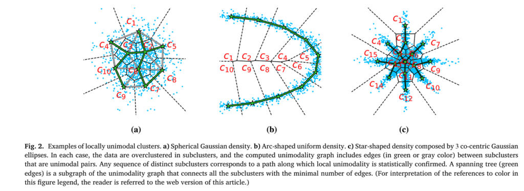
UniForCE flips this paradigm. Instead of requiring the entire cluster to be unimodal, it introduces the concept of a Locally Unimodal Cluster.
A cluster is locally unimodal if it can be broken down into smaller, homogeneous subclusters such that unimodality is preserved between any connected pair of these subclusters.
Think of it like building a bridge: you don’t need to see the entire structure from one point; you just need to ensure that each segment connects solidly to the next. This local criterion allows UniForCE to identify much more complex cluster geometries.
How UniForCE Works: A Three-Step Pipeline
The UniForCE methodology is an elegant bottom-up aggregation process, visualized in the diagram below. It consists of three main stages.
% Image Description: A flowchart illustrating the three main steps of the UniForCE algorithm.
% Step 1: A scatter plot of a complex 2D dataset with multiple irregular shapes inside a ring.
% Step 2: The same data, now overclustered into many small, colored groups using k-means.
% Step 3: A graph where each subcluster is a node, and green edges connect unimodal pairs. A Minimum Spanning Forest is computed, defining the final clusters.
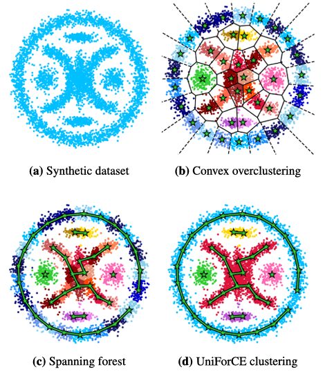
Step 1: Intelligent Overclustering
The process begins by overclustering the dataset into a large number K (e.g., 50) of small, homogeneous subclusters. This is typically done using an algorithm like *k*-means++, which creates subclusters that lie in convex regions.
- Why overcluster? This initial step breaks the complex clustering problem into many simpler, local problems. It’s like breaking a large mosaic into its individual tiles before reassembling them into the correct image.
- Robustness: The algorithm uses a variant called global *k*-means++ to ensure a high-quality initialization even for a large K. Subclusters with very few points are eliminated and reassigned to ensure each subcluster has enough data points (a minimum of M=25) for valid statistical testing in the next step.
Step 2: Unimodal Pair Testing – The Statistical Heart
This is the most innovative part of UniForCE. The algorithm tests pairs of neighboring subclusters to decide if their union is unimodal.
- Projection: For two subclusters ci and cj, with centers μi and μj, UniForCE finds the perpendicular bisecting hyperplane Hij between the centers.
- Distance Calculation: It calculates the signed distance of every data point in the two subclusters to this hyperplane, creating a one-dimensional set of distances, Pij.
- The Dip Test: It applies Hartigans’ dip-test, a powerful statistical test for unimodality, to this 1D set Pij. If the test does not reject the null hypothesis of unimodality (i.e., the p-value is above a significance level αα, e.g., 0.001), the pair is declared a unimodal pair.
Handling Imbalance: A key refinement addresses imbalanced subclusters. If one subcluster is much larger, the dip-test might incorrectly declare a multimodal distribution as unimodal. UniForCE solves this by taking a balanced random sample from the larger subcluster for the test, repeating the process multiple times (a Monte Carlo simulation), and using a majority vote for a robust decision.
Step 3: Building the Unimodality Forest
The results of the pairwise tests are used to build a unimodality graph:
- Vertices: Each subcluster from the overclustering.
- Edges: An edge connects two vertices if their corresponding subclusters form a unimodal pair.
The final clusters are simply the connected components of this graph. If you can travel from one subcluster to another via a path of unimodal pairs, they belong to the same final cluster. UniForCE efficiently computes a Minimum Spanning Forest (MSF) of this graph, where each tree in the forest represents a maximal locally unimodal cluster. The number of trees is the estimated number of clusters kk.
Experimental Evidence: Outperforming the State-of-the-Art
The UniForCE method was rigorously tested against a battery of other clustering algorithms on both real and synthetic datasets. The competitors included:
- Top-down statistical methods: X-means, G-means, PG-means, Dip-means.
- Density-based methods: HDBSCAN, Mean Shift.
- Other modern approaches: RCC, SMMP.
Performance was measured using Adjusted Mutual Information (AMI) and Adjusted Rand Index (ARI), which evaluate how well the algorithm’s output matches the ground-truth labels (higher is better), along with the accuracy of the estimated kk.
Key Results on Real Data
The following table summarizes the performance on a selection of challenging real-world datasets, including handwritten digits (EMNIST), human activity recognition (HAR), and cancer gene data (TCGA).
| Dataset (True k) | UniForCE (k, AMI, ARI) | Best Competitor (k, AMI, ARI) | Key Takeaway |
|---|---|---|---|
| EMNIST-BD (k=10) | 10, 0.87, 0.87 | Dip-means (7, 0.60, 0.53) | UniForCE correctly finds 10 clusters with high accuracy, while others fail. |
| YTF Faces (k=40) | 39, 0.94, 0.89 | HDBSCAN (50, 0.91, 0.83) | Excellent performance on a complex image dataset. |
| Waveform-v1 (k=3) | 3, 1.00, 1.00 | RCC (3, 1.00, 1.00) | Perfect results, matching the best competitor. |
| TCGA Cancer (k=5) | 5, 0.93, 0.94 | RCC (8, 0.84, 0.85) | Superior clustering that matches the biological classes. |
| Mice Protein (k=8) | 8, 0.93, 0.91 | HDBSCAN (11, 0.93, 0.95) | Highly accurate, with a nearly perfect kk estimate. |
The consensus was clear: UniForCE consistently provided accurate estimates of k and high-quality clustering results across a diverse range of datasets, outperforming methods that rely on stricter assumptions like Gaussianity.
Mastering Complex Shapes on Synthetic Data
On synthetic 2D and 3D datasets designed to stress-test clustering algorithms—featuring rings, spirals, elongated curves, and nested clusters—UniForCE demonstrated remarkable versatility. The locally unimodal cluster definition proved flexible enough to capture this wide variety of densities and shapes where traditional methods often break down.
Discussion: The Strengths and Limitations of UniForCE
Why UniForCE is a Significant Advancement
- Statistically Sound Foundation: Unlike heuristic merging criteria, UniForCE uses a formal statistical test (the dip-test) to guide cluster aggregation. This provides a principled, non-parametric foundation for the algorithm.
- Automatic k Estimation: The number of clusters emerges naturally from the data structure via the connected components of the unimodality graph, eliminating the need for manual input or complex validation indices.
- Flexibility for Arbitrary Shapes: The local unimodality criterion allows it to identify highly complex cluster structures that are not globally unimodal, convex, or linearly separable.
- Robustness to Hyperparameters: A sensitivity analysis showed that UniForCE performs consistently well across a wide range of its hyperparameter settings (K, α, L, M), making it practical for real-world use.
Practical Considerations and Limitations
No algorithm is perfect, and understanding its boundaries is key to effective application.
- Overclustering Resolution: The initial number of subclusters KK sets a lower bound on the resolution of discoverable clusters. Clusters smaller than the initial subclusters cannot be identified.
- Focus on Shape, Not Density Level: UniForCE focuses on the shape of the density (unimodality) rather than its absolute level. Intensive noise between two true clusters could, in theory, create bridging subclusters that lead to under-estimation of k.
- Computational Cost: While optimized, the pairwise testing can be more computationally intensive than simpler methods like *k*-means, especially for very large K.
In practice, these limitations can often be mitigated by standard preprocessing (denoising) and by using the recommended default parameters, which have been shown to be effective across many datasets.
Conclusion and Future Directions
UniForCE represents a paradigm shift in clustering by leveraging local unimodality—a simple yet powerful statistical property—to solve the dual problems of clustering and cluster count estimation. Its ability to uncover complex structures in a statistically rigorous and automatic fashion makes it a valuable tool for data scientists facing the challenge of exploring unlabeled data.
The concept of testing properties locally, rather than globally, opens up exciting avenues for future research. This principle could be extended to other unsupervised learning tasks like dimensionality reduction, density estimation, and anomaly detection. Furthermore, developing new cluster validation indices tailored for assessing irregular-shaped clusters would complement methodologies like UniForCE and deepen our understanding of cluster quality.
Call to Action: Explore and Engage
Are you wrestling with a complex clustering problem in your work? The principles behind UniForCE—local assessment, statistical testing, and bottom-up aggregation—can provide a fresh perspective, even if you don’t use the algorithm directly.
- Try UniForCE: The source code is publicly available on GitHub (see the research paper for the link).
- Re-evaluate Your Assumptions: The next time you reach for a standard clustering algorithm, consider your cluster assumption. Is your data really composed of spherical blobs?
- Share Your Experience: Have you used advanced clustering methods like HDBSCAN or Dip-means? What challenges have you faced? Join the conversation in the comments below.
Deepen your understanding of machine learning fundamentals. Subscribe to our newsletter for more insightful breakdowns of cutting-edge research and practical data science techniques.
Below is the complete code, which encapsulates the entire workflow described in the paper. This includes the initial overclustering, the unimodal pair testing using Hartigans’ dip-test, and the final cluster aggregation via a spanning forest. The code is structured to be self-contained and includes comments explaining each part of the process, from data preprocessing to the final cluster assignment.
# -*- coding: utf-8 -*-
"""
UniForCE: The Unimodality Forest method for Clustering and Estimation of the number of clusters.

This script provides an implementation of the UniForCE algorithm as described in the paper
by Georgios Vardakas, Argyris Kalogeratos, and Aristidis Likas.

The algorithm works in three main stages:
1. Overclustering: The dataset is initially partitioned into a large number of small,
   homogeneous subclusters using an incremental k-means++ approach. Small subclusters
   are eliminated.
2. Unimodal Pair Testing: A statistical test is used to determine if the union of any
   two subclusters is unimodal. This is the core of the method and helps define a
   "unimodality graph".
3. Clustering by Aggregation: A minimum spanning forest is computed on the graph of
   subclusters, where edge weights are distances, but edges are only added if the
   corresponding subcluster pair passes the unimodal pair test. The trees in the
   final forest represent the final clusters.
"""

import numpy as np
from sklearn.cluster import KMeans
from sklearn.metrics.pairwise import euclidean_distances
from scipy.spatial.distance import cdist
from diptest import diptest # Requires `pip install diptest`

class UniForCE:
    """
    Implementation of the Unimodality Forest for Clustering and Estimation (UniForCE) algorithm.

    Parameters
    ----------
    K_prime : int, default=50
        The initial number of subclusters for the overclustering step. Should be
        significantly larger than the expected number of true clusters.
    M : int, default=25
        The minimum number of data points a subcluster must have to be considered.
        Subclusters smaller than this are merged into their nearest neighbors.
    L : int, default=11
        The number of Monte Carlo simulations for the unimodal pair test. Must be odd.
    alpha : float, default=0.001
        The significance level for the Hartigans' dip-test for unimodality.
        A pair of subclusters is considered jointly unimodal if the p-value > alpha.

    Attributes
    ----------
    labels_ : ndarray of shape (n_samples,)
        Cluster labels for each point in the dataset given to fit().
    n_clusters_ : int
        The estimated number of clusters found by the algorithm.
    """
    def __init__(self, K_prime=50, M=25, L=11, alpha=0.001):
        if not isinstance(K_prime, int) or K_prime <= 0:
            raise ValueError("K_prime must be a positive integer.")
        if not isinstance(M, int) or M <= 0:
            raise ValueError("M must be a positive integer.")
        if not (isinstance(L, int) and L > 0 and L % 2 != 0):
            raise ValueError("L must be a positive odd integer.")
        if not (isinstance(alpha, float) and 0 < alpha < 1):
            raise ValueError("alpha must be a float between 0 and 1.")

        self.K_prime = K_prime
        self.M = M
        self.L = L
        self.alpha = alpha

        self.labels_ = None
        self.n_clusters_ = None

    def _global_kmeans_pp(self, X, n_clusters):
        """
        Performs an incremental version of k-means++ for robust overclustering.
        This is a simplified version of the global k-means++ idea.
        """
        centers = np.empty((n_clusters, X.shape[1]))

        # First center is chosen randomly
        centers[0] = X[np.random.choice(X.shape[0])]

        for i in range(1, n_clusters):
            dist_sq = np.min(cdist(X, centers[:i], 'sqeuclidean'), axis=1)
            probs = dist_sq / np.sum(dist_sq)
            # Use np.random.multinomial to handle the case of duplicate points
            # which could cause issues with np.random.choice
            cumulative_probs = probs.cumsum()
            r = np.random.rand()
            new_center_idx = np.searchsorted(cumulative_probs, r)
            centers[i] = X[new_center_idx]

        kmeans = KMeans(n_clusters=n_clusters, init=centers, n_init=1).fit(X)
        return kmeans.labels_, kmeans.cluster_centers_

    def _preprocess(self, X, labels, centers):
        """
        Removes subclusters smaller than M and reassigns their points.
        """
        unique_labels, counts = np.unique(labels, return_counts=True)

        small_clusters = unique_labels[counts < self.M]

        while len(small_clusters) > 0:
            current_labels = np.unique(labels)
            valid_centers_mask = np.isin(current_labels, small_clusters, invert=True)
            valid_centers = centers[valid_centers_mask]

            for small_clust_label in small_clusters:
                points_to_reassign = X[labels == small_clust_label]
                if points_to_reassign.shape[0] == 0:
                    continue

                # Find nearest valid center for these points
                distances = cdist(points_to_reassign, valid_centers)
                nearest_center_indices = np.argmin(distances, axis=1)

                # Map back to original label indices
                original_labels = current_labels[valid_centers_mask]
                new_labels_for_points = original_labels[nearest_center_indices]

                labels[labels == small_clust_label] = new_labels_for_points

            unique_labels, counts = np.unique(labels, return_counts=True)
            small_clusters = unique_labels[counts < self.M]

        # Re-map labels to be contiguous from 0 to K-1
        final_labels_unique = np.unique(labels)
        label_map = {old_label: new_label for new_label, old_label in enumerate(final_labels_unique)}
        final_labels = np.array([label_map[l] for l in labels])

        # Recalculate centers for the final set of clusters
        final_centers = np.array([X[final_labels == i].mean(axis=0) for i in range(len(final_labels_unique))])

        return final_labels, final_centers

    def _is_unimodal_pair(self, c_i, c_j, mu_i, mu_j):
        """
        Performs the unimodal pair test as described in Algorithm 2 of the paper.
        """
        if c_i.shape[0] > c_j.shape[0]:
            c_i, c_j = c_j, c_i  # Ensure c_i is the smaller cluster

        # Define the perpendicular bisecting hyperplane
        r_ij = mu_j - mu_i
        midpoint = (mu_i + mu_j) / 2

        # Handle case where centers are identical
        if np.linalg.norm(r_ij) == 0:
            return True # They are effectively the same point, so unimodal

        def get_signed_distances(points, w, b):
            return (points @ w + b) / np.linalg.norm(w)

        # Hyperplane: w^T * x + b = 0, where w = r_ij and b = -r_ij^T * midpoint
        w = r_ij
        b = -np.dot(r_ij, midpoint)

        # Get signed distances for the smaller cluster
        dists_i = get_signed_distances(c_i, w, b)

        votes_for_unimodality = 0
        for _ in range(self.L):
            # Subsample the larger cluster
            indices = np.random.choice(c_j.shape[0], c_i.shape[0], replace=False)
            c_j_sample = c_j[indices]

            dists_j = get_signed_distances(c_j_sample, w, b)

            all_dists = np.concatenate((dists_i, dists_j))

            # Perform Hartigans' dip-test
            p_value = diptest(all_dists, boot_p=False)[1] # We only need the p-value

            if p_value >= self.alpha:
                votes_for_unimodality += 1

        # Decide based on majority vote
        return votes_for_unimodality > self.L / 2

    def fit(self, X):
        """
        Performs clustering on the dataset X.

        Parameters
        ----------
        X : array-like of shape (n_samples, n_features)
            The input data to cluster.
        """
        print("1. Starting overclustering...")
        # Step 1: Overclustering
        initial_labels, initial_centers = self._global_kmeans_pp(X, self.K_prime)

        print("2. Preprocessing subclusters (removing small ones)...")
        # Preprocessing: remove small clusters
        subcluster_labels, subcluster_centers = self._preprocess(X, initial_labels, initial_centers)

        K = len(subcluster_centers)
        print(f"   Overclustering resulted in {K} subclusters after preprocessing.")

        subclusters = [X[subcluster_labels == i] for i in range(K)]

        print("3. Building unimodality spanning forest...")
        # Step 2 & 3: Build spanning forest using a Kruskal-like approach

        # Calculate pairwise distances between subcluster centers
        distances = euclidean_distances(subcluster_centers)

        # Create a list of edges (distance, i, j) for all pairs i < j
        edges = []
        for i in range(K):
            for j in range(i + 1, K):
                edges.append((distances[i, j], i, j))

        # Sort edges by distance
        edges.sort()

        # Disjoint Set Union (DSU) for tracking connected components (trees)
        parent = list(range(K))
        def find(i):
            if parent[i] == i:
                return i
            parent[i] = find(parent[i])
            return parent[i]

        def union(i, j):
            root_i = find(i)
            root_j = find(j)
            if root_i != root_j:
                parent[root_j] = root_i

        num_edges_added = 0
        for i, (dist, u, v) in enumerate(edges):
            if find(u) != find(v):
                # Only test if they are in different trees
                is_unimodal = self._is_unimodal_pair(
                    subclusters[u], subclusters[v],
                    subcluster_centers[u], subcluster_centers[v]
                )
                if is_unimodal:
                    union(u, v)
                    num_edges_added += 1

            if (i+1) % 100 == 0:
                print(f"   Processed {i+1}/{len(edges)} potential edges...")

            if num_edges_added == K -1: # Optimization: forest cannot have more edges
                break

        print("4. Assigning final cluster labels...")
        # Final cluster assignment
        final_cluster_map = {i: find(i) for i in range(K)}

        # Map root labels to 0, 1, 2, ...
        root_labels = np.unique(list(final_cluster_map.values()))
        self.n_clusters_ = len(root_labels)
        root_map = {old_label: new_label for new_label, old_label in enumerate(root_labels)}

        # Assign final labels to data points
        self.labels_ = np.zeros(X.shape[0], dtype=int)
        for i in range(K):
            root = final_cluster_map[i]
            final_label = root_map[root]
            self.labels_[subcluster_labels == i] = final_label

        print(f"Done. Estimated number of clusters: {self.n_clusters_}")
        return self

# Example Usage
if __name__ == '__main__':
    from sklearn.datasets import make_blobs, make_moons
    from sklearn.metrics import adjusted_rand_score, adjusted_mutual_info_score
    import matplotlib.pyplot as plt

    print("--- Running UniForCE on a simple blobs dataset ---")
    X_blobs, y_blobs = make_blobs(n_samples=1000, centers=4, n_features=2, cluster_std=0.8, random_state=42)

    uniforce_blobs = UniForCE(K_prime=30, M=15, alpha=0.01)
    uniforce_blobs.fit(X_blobs)

    ari_blobs = adjusted_rand_score(y_blobs, uniforce_blobs.labels_)
    ami_blobs = adjusted_mutual_info_score(y_blobs, uniforce_blobs.labels_)

    print(f"\nResults for Blobs Dataset:")
    print(f"True number of clusters: 4")
    print(f"Estimated number of clusters: {uniforce_blobs.n_clusters_}")
    print(f"Adjusted Rand Index (ARI): {ari_blobs:.4f}")
    print(f"Adjusted Mutual Information (AMI): {ami_blobs:.4f}")

    plt.figure(figsize=(12, 5))
    plt.subplot(1, 2, 1)
    plt.scatter(X_blobs[:, 0], X_blobs[:, 1], c=y_blobs, cmap='viridis', s=10)
    plt.title("Ground Truth (Blobs)")
    plt.xlabel("Feature 1")
    plt.ylabel("Feature 2")

    plt.subplot(1, 2, 2)
    plt.scatter(X_blobs[:, 0], X_blobs[:, 1], c=uniforce_blobs.labels_, cmap='viridis', s=10)
    plt.title(f"UniForCE Result (k={uniforce_blobs.n_clusters_})")
    plt.xlabel("Feature 1")
    plt.ylabel("Feature 2")
    plt.suptitle("UniForCE on Blobs Dataset")
    plt.tight_layout(rect=[0, 0, 1, 0.96])
    plt.show()

    print("\n--- Running UniForCE on a non-convex (moons) dataset ---")
    X_moons, y_moons = make_moons(n_samples=1000, noise=0.05, random_state=42)

    # Non-convex shapes often require a finer overclustering
    uniforce_moons = UniForCE(K_prime=50, M=10, alpha=0.001)
    uniforce_moons.fit(X_moons)

    ari_moons = adjusted_rand_score(y_moons, uniforce_moons.labels_)
    ami_moons = adjusted_mutual_info_score(y_moons, uniforce_moons.labels_)

    print(f"\nResults for Moons Dataset:")
    print(f"True number of clusters: 2")
    print(f"Estimated number of clusters: {uniforce_moons.n_clusters_}")
    print(f"Adjusted Rand Index (ARI): {ari_moons:.4f}")
    print(f"Adjusted Mutual Information (AMI): {ami_moons:.4f}")

    plt.figure(figsize=(12, 5))
    plt.subplot(1, 2, 1)
    plt.scatter(X_moons[:, 0], X_moons[:, 1], c=y_moons, cmap='viridis', s=10)
    plt.title("Ground Truth (Moons)")
    plt.xlabel("Feature 1")
    plt.ylabel("Feature 2")

    plt.subplot(1, 2, 2)
    plt.scatter(X_moons[:, 0], X_moons[:, 1], c=uniforce_moons.labels_, cmap='viridis', s=10)
    plt.title(f"UniForCE Result (k={uniforce_moons.n_clusters_})")
    plt.xlabel("Feature 1")
    plt.ylabel("Feature 2")
    plt.suptitle("UniForCE on Moons Dataset")
    plt.tight_layout(rect=[0, 0, 1, 0.96])
    plt.show()
Related posts, You May like to read
- 7 Shocking Truths About Knowledge Distillation: The Good, The Bad, and The Breakthrough (SAKD)
- 7 Revolutionary Breakthroughs in Medical Image Translation (And 1 Fatal Flaw That Could Derail Your AI Model)
- DeepSPV: Revolutionizing 3D Spleen Volume Estimation from 2D Ultrasound with AI
- ACAM-KD: Adaptive and Cooperative Attention Masking for Knowledge Distillation
- GeoSAM2 3D Part Segmentation — Prompt-Controllable, Geometry-Aware Masks for Precision 3D Editing
- Probabilistic Smooth Attention for Deep Multiple Instance Learning in Medical Imaging
- A Knowledge Distillation-Based Approach to Enhance Transparency of Classifier Models
- Towards Trustworthy Breast Tumor Segmentation in Ultrasound Using AI Uncertainty
- Discrete Migratory Bird Optimizer with Deep Transfer Learning for Multi-Retinal Disease Detection