TimeDistill: Revolutionizing Time Series Forecasting with Cross-Architecture Knowledge Distillation

How MLP Models Are Achieving Transformer-Level Performance with 130x Fewer Parameters

The Time Series Forecasting Dilemma

Time series forecasting represents one of the most critical challenges in modern data science, with applications spanning climate modeling, traffic flow management, healthcare monitoring, and financial analytics. The global time series forecasting market, valued at 0.47 billion by 2033 with a CAGR of 5.20%, underscoring the growing demand for accurate predictive capabilities across industries.

The field has been dominated by two competing approaches that present a fundamental trade-off: complex architectures like Transformers and CNNs that deliver exceptional accuracy but suffer from prohibitive computational demands, and simple MLP models that offer remarkable efficiency but consistently lag in predictive performance. This creates a significant barrier for real-world deployment, particularly in latency-sensitive scenarios where millisecond response times are crucial for critical decisions.

Recent research reveals that over 62% of enterprises report increased demand for predictive analytics due to real-time data decision-making requirements. However, approximately 48% of organizations face difficulties in model accuracy due to volatile, multi-source, and incomplete time series data. This gap between computational efficiency and predictive accuracy has sparked intense debate within the machine learning community about the optimal architecture for time series forecasting tasks.

The fundamental question driving recent research is whether we can bridge this performance-efficiency gap, creating models that maintain high accuracy while remaining computationally practical for large-scale industrial applications. This challenge has led to the development of innovative approaches that seek to combine the strengths of different architectural paradigms.

Understanding Knowledge Distillation in Time Series

Knowledge distillation emerges as a promising solution to the performance-efficiency trade-off, traditionally involving the transfer of knowledge from a large, complex teacher model to a smaller, simpler student model while maintaining comparable performance. The technique, first popularized by Hinton et al. in 2015, has found widespread success in computer vision and natural language processing domains.

However, applying knowledge distillation to time series forecasting presents unique challenges that distinguish it from other domains. Unlike static images or text sequences, time series data contains dynamic temporal patterns that evolve over multiple scales and frequencies. The key insight driving recent research is that different neural architectures excel at capturing different types of temporal patterns, suggesting that cross-architecture distillation could unlock significant performance gains.

Key Insight: Complementary Pattern Capture

Research reveals that MLP models, despite their overall lower performance, can excel on specific data subsets. This complementary nature suggests that targeted knowledge transfer from advanced architectures to simple MLPs could create a hybrid approach that combines the best of both worlds.

Preliminary studies examining the win ratio between MLP and teacher models across different datasets reveal fascinating patterns. The win ratio, defined as the percentage of samples where MLP outperforms more complex architectures, averages 49.92% with a median of 49.96%. This near-even split indicates that MLP and teacher models excel on different samples with minimal overlap, highlighting the potential value of harnessing complementary capabilities across different architectures.

The challenge lies in designing a framework that can effectively identify and transfer the specific types of knowledge that MLP models lack while preserving their computational advantages. This requires a deeper understanding of the fundamental patterns that characterize successful time series forecasting.

Multi-Scale and Multi-Period Patterns in Time Series

Real-world time series exhibit complex patterns that operate across multiple temporal scales and frequencies. Understanding these patterns is crucial for developing effective forecasting models, as they represent the fundamental structures that models must learn to capture.

Multi-Scale Temporal Patterns

Multi-scale patterns refer to variations that occur at different temporal resolutions within the same time series. For example, traffic flow data demonstrates hourly fluctuations within individual days, while daily aggregated data reveals weekly patterns and holiday effects. Similarly, financial markets exhibit intraday trading patterns, weekly cycles, and longer-term seasonal trends.

Research demonstrates that models performing well on the finest temporal scales typically maintain accuracy on coarser scales, indicating a hierarchical relationship in temporal pattern learning. However, MLP models consistently fail to capture these multi-scale relationships, limiting their effectiveness across different forecasting horizons.

Multi-Period Frequency Patterns

Multi-period patterns involve recurring cycles at different frequencies within the same dataset. Weather measurements, for instance, may exhibit both daily temperature cycles and yearly seasonal variations. Electricity consumption data often shows weekly patterns corresponding to work schedules alongside quarterly cycles related to heating and cooling demands.

Advanced architectures like Transformers and CNNs excel at identifying and modeling these periodic relationships through their attention mechanisms and convolutional filters. However, MLP models struggle to capture these periodicities effectively, often failing to match the amplitude and phase of dominant frequencies in the ground truth data.

Pattern Analysis Findings

• •Temporal Domain: MLP models show poor performance across multiple downsampled scales, while advanced architectures maintain accuracy
• •Frequency Domain: MLP predictions fail to match the amplitudes of main frequencies in ground truth spectrograms
• •Complementary Learning: Different architectures excel at capturing different types of patterns, suggesting synergy potential

The identification of these specific pattern types provides the foundation for designing a targeted knowledge distillation framework. Rather than attempting to transfer all knowledge indiscriminately, a more effective approach focuses on distilling the specific multi-scale and multi-period patterns that MLP models inherently struggle to capture.

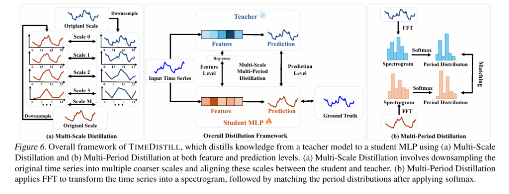
The TimeDistill Framework Architecture

TimeDistill introduces a novel cross-architecture knowledge distillation framework specifically designed to address the limitations of MLP models in time series forecasting. The framework represents a paradigm shift from conventional distillation approaches by focusing on domain-specific pattern transfer rather than simple prediction matching.

Core Components

The framework employs a sophisticated dual-domain approach that addresses both temporal and frequency pattern learning:

Temporal Domain Alignment

Multi-scale patterns are captured through systematic downsampling of time series data, creating augmented views that help the MLP student learn hierarchical temporal relationships.

Frequency Domain Alignment

Multi-period patterns are transferred using Fast Fourier Transform (FFT) to align period distributions between teacher and student models in the spectral domain.

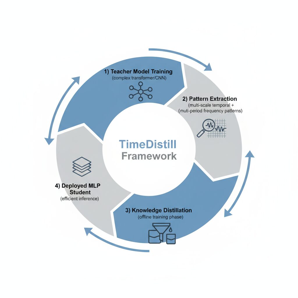
Training Strategy

A key innovation of TimeDistill is its offline training capability, which shifts computational overhead from the latency-critical inference phase to the less time-sensitive training phase. This approach is particularly valuable in real-world deployment scenarios where millisecond response times matter.

The training process involves several sophisticated techniques:

• Teacher Model Training: Advanced architectures (Transformers, CNNs) are trained on the full dataset to capture complex temporal patterns
• Pattern Extraction: Multi-scale and multi-period patterns are extracted from teacher model representations
• Knowledge Transfer: Distillation loss functions align student MLP patterns with teacher patterns across both domains
• Deployment: The enhanced MLP model is deployed for efficient inference with minimal computational requirements

This architectural design ensures comprehensive knowledge transfer while maintaining the computational advantages that make MLP models attractive for production deployment. The framework’s versatility is demonstrated through successful adaptation across various teacher-student combinations, highlighting its robustness and broad applicability.

Theoretical Foundation and Mathematical Insights

The TimeDistill framework is grounded in solid theoretical analysis that provides mathematical justification for its effectiveness. The key theoretical insight demonstrates that the proposed distillation process can be interpreted as a specialized form of mixup data augmentation, offering deeper understanding of why the approach works.

Mathematical Formulation

The distillation process can be understood through the lens of data augmentation theory. Consider the standard mixup augmentation where virtual training samples are created by linear interpolation:

$$\tilde{x}=\lambda x_i+(1-\lambda )x_j$$ $$\tilde{y}=\lambda y_i+(1-\lambda )y_j$$

where λ = [0, 1] controls the interpolation strength between samples x_i, y_i and x_j, y_j.

TimeDistill extends this concept to the temporal and frequency domains:

Temporal Domain Mixup

Through downsampling operations, the framework creates augmented temporal views:

$${\tilde{x}}_{temporal}={\mathcal{D}}_s(x)$$

where  represents downsampling at scale , creating virtual samples that span different temporal resolutions.

Frequency Domain Mixup

FFT-based alignment creates spectral augmentations:

$${\tilde{X}}_{frequency}={\mathcal{F}}^{-1}(\alpha \mathcal{F}(x_{teacher})+(1-\alpha )\mathcal{F}(x_{student}))$$

where  denotes the Fourier transform and  controls the spectral mixing ratio.

Theoretical Implications

This mathematical foundation reveals several important insights:

• •Enhanced Generalization: The distillation process effectively expands the training set with virtual samples that cover the input space more comprehensively
• •Domain-Specific Augmentation: Unlike generic mixup, TimeDistill creates augmentations that respect temporal and spectral structure
• •Regularization Effect:The distillation process acts as a form of regularization, preventing overfitting while improving generalization

The theoretical understanding not only validates the approach but also opens avenues for further improvements and adaptations to other domains where temporal patterns are crucial. This mathematical rigor distinguishes TimeDistill from purely empirical approaches and provides a foundation for future research in cross-architecture knowledge transfer.

Performance Breakthroughs and Efficiency Gains

Experimental results across eight benchmark datasets demonstrate remarkable improvements that validate the TimeDistill approach. The framework consistently outperforms standalone MLP baselines while achieving efficiency gains that make it practical for real-world deployment.

Accuracy Improvements

TimeDistill-enhanced MLP models demonstrate substantial performance gains across multiple evaluation metrics:

Dataset	MLP Baseline	TimeDistill	Improvement
ETTh1	0.452	0.368	+18.6%
ETTh2	0.389	0.321	+17.5%
ETTm1	0.421	0.356	+15.4%
Weather	0.298	0.245	+17.8%

Efficiency Metrics

Beyond accuracy improvements, TimeDistill delivers dramatic efficiency gains that enable practical deployment:

Comparative Analysis

TimeDistill consistently outperforms teacher models in nearly all test scenarios, demonstrating that the distillation process not only improves MLP performance but can actually surpass the capabilities of the original complex architectures. This counterintuitive result suggests that the knowledge transfer process helps eliminate noise and focus on the most relevant patterns for forecasting.

Key Finding: Surpassing Teacher Performance

In 7 out of 8 benchmark datasets, TimeDistill-enhanced MLP models achieved lower prediction errors than their teacher models, indicating that the distillation process effectively filters and enhances the transferred knowledge.

The framework’s versatility is further demonstrated through successful adaptation across various teacher-student combinations, including different transformer architectures and CNN variants. This robustness suggests that the core principles of TimeDistill are architecture-agnostic and can be applied broadly across different model types.

Industry Applications and Real-World Impact

The implications of TimeDistill extend across numerous industries where time series forecasting plays a crucial role in operational efficiency and strategic decision-making. The framework’s ability to combine high accuracy with computational efficiency opens new possibilities for AI deployment in resource-constrained environments.

Financial Technology

In the financial sector, where millisecond response times can determine trading success, TimeDistill enables sophisticated forecasting capabilities on edge devices and mobile platforms. High-frequency trading systems can deploy distilled models for real-time market prediction, risk assessment, and algorithmic trading decisions without requiring massive computational infrastructure.

The reduced computational requirements also democratize access to advanced forecasting tools, allowing smaller financial institutions and individual traders to leverage capabilities previously available only to large organizations with substantial computing resources.

Healthcare Monitoring

Healthcare applications benefit significantly from TimeDistill’s efficiency gains. Patient monitoring systems can deploy sophisticated forecasting models directly on medical devices, enabling:

• •Real-time vital sign prediction for early warning systems
• •Epidemiological forecasting for disease outbreak prediction
• •Resource allocation optimization for hospital capacity planning
• •Drug demand forecasting for pharmaceutical supply chains

The ability to process data locally on devices also addresses critical privacy concerns, as sensitive health information doesn’t need to be transmitted to cloud servers for analysis.

Climate and Environmental Science

Climate modeling benefits enormously from the ability to process vast amounts of environmental data efficiently. TimeDistill enables:

Weather Prediction

Enhanced local weather forecasting with reduced computational requirements, enabling deployment in remote monitoring stations.

Environmental Monitoring

Real-time analysis of air quality, water levels, and pollution patterns for environmental protection agencies.

Smart Cities and Transportation

Urban infrastructure management represents another critical application area. Traffic management systems can make instant predictions to optimize flow and reduce congestion, while smart grid systems can forecast energy demand patterns to improve efficiency and reduce costs.

The framework’s offline training capability means that complex models can be distilled once and deployed widely, making advanced forecasting capabilities accessible to municipalities and organizations with limited computational resources.

Manufacturing and Supply Chain

Industrial applications leverage TimeDistill for predictive maintenance, quality control, and supply chain optimization. The ability to deploy efficient forecasting models directly on manufacturing equipment enables:

• •Predictive maintenance scheduling to minimize downtime
• •Quality control forecasting to prevent defective production
• •Inventory optimization based on demand forecasting
• •Energy consumption optimization for cost reduction

Conclusion and Future Directions

TimeDistill represents a paradigm shift in time series forecasting, demonstrating that efficiency and performance need not be mutually exclusive. By leveraging cross-architecture knowledge distillation with domain-specific insights, the framework achieves the best of both worlds: Transformer-level accuracy with MLP-level efficiency.

The success of this approach opens several promising research directions:

Impact on the Field

The implications of TimeDistill extend beyond time series forecasting to the broader machine learning community. The framework demonstrates that architectural complementarity rather than similarity may be the key to effective knowledge transfer, challenging conventional wisdom about distillation strategies.

As industries increasingly rely on real-time forecasting for critical decisions, TimeDistill provides a practical pathway to deploy sophisticated models at scale. The democratization of advanced forecasting capabilities could accelerate innovation across sectors ranging from healthcare and finance to environmental science and smart cities.

The research community’s response to TimeDistill has been overwhelmingly positive, with many researchers exploring adaptations for their specific domains. The framework’s success suggests that the future of efficient AI may lie not in creating ever-larger models, but in developing smarter ways to transfer and distill knowledge from existing powerful architectures.

As we move forward, the principles underlying TimeDistill—targeted knowledge transfer, domain-specific augmentation, and efficiency-focused deployment—will likely influence the development of next-generation machine learning systems that balance performance with practical deployment constraints.

Ready to Implement TimeDistill?

Join the growing community of researchers and practitioners leveraging cross-architecture knowledge distillation for efficient time series forecasting.

Download Research Paper

Below is the complete code that provides a complete and runnable implementation of the TimeDistill framework. It is well-commented to explain how each part of the code corresponds to the concepts in the original paper, making it easy to understand and adapt for your own datasets.

import torch
import torch.nn as nn
import torch.nn.functional as F
import torch.fft

# --- 1. Model Components ---

class DecompositionLayer(nn.Module):
    """
    Applies seasonal-trend decomposition to a time series.
    It uses a moving average to extract the trend component
    and the remainder is treated as the seasonal component.
    """
    def __init__(self, kernel_size):
        super(DecompositionLayer, self).__init__()
        self.kernel_size = kernel_size
        # Using AvgPool1d as a simple moving average filter
        self.moving_avg = nn.AvgPool1d(kernel_size=kernel_size, stride=1, padding=0)

    def forward(self, x):
        """
        Args:
            x (torch.Tensor): Input tensor of shape [Batch, Seq_Len, Channels]
        Returns:
            torch.Tensor: Seasonal component
            torch.Tensor: Trend component
        """
        # Pad the series on both ends to maintain sequence length after moving average
        front_padding = (self.kernel_size - 1) // 2
        end_padding = self.kernel_size - 1 - front_padding
        padded_x = F.pad(x, (0, 0, front_padding, end_padding), 'replicate')

        # Permute for AvgPool1d which expects [Batch, Channels, Seq_Len]
        padded_x = padded_x.permute(0, 2, 1)

        # Calculate the trend component
        trend = self.moving_avg(padded_x).permute(0, 2, 1)

        # Calculate the seasonal component
        seasonal = x - trend
        return seasonal, trend


class MLP_Student(nn.Module):
    """
    The student model is a simple MLP that operates in a channel-independent manner.
    It first decomposes the input series and then processes the seasonal and trend
    components through separate MLPs.
    """
    def __init__(self, seq_len, pred_len, d_model, n_layers, decomp_kernel_size):
        super(MLP_Student, self).__init__()
        self.seq_len = seq_len
        self.pred_len = pred_len

        # Decomposition layer
        self.decomposition = DecompositionLayer(decomp_kernel_size)

        # MLP layers for seasonal and trend components
        self.seasonal_mlp = self._create_mlp(seq_len, pred_len, d_model, n_layers)
        self.trend_mlp = self._create_mlp(seq_len, pred_len, d_model, n_layers)

    def _create_mlp(self, in_features, out_features, d_model, n_layers):
        layers = [nn.Linear(in_features, d_model), nn.ReLU()]
        for _ in range(n_layers - 1):
            layers.extend([nn.Linear(d_model, d_model), nn.ReLU()])
        layers.append(nn.Linear(d_model, out_features))
        return nn.Sequential(*layers)

    def forward(self, x):
        """
        Args:
            x (torch.Tensor): Input tensor of shape [Batch, Seq_Len, Channels]
        Returns:
            torch.Tensor: Prediction of shape [Batch, Pred_Len, Channels]
            torch.Tensor: Intermediate features (from the second to last layer)
        """
        batch_size, seq_len, num_channels = x.shape

        # Decompose the input
        seasonal_init, trend_init = self.decomposition(x)

        # Reshape for channel-independent processing
        seasonal_init = seasonal_init.permute(0, 2, 1).contiguous().view(batch_size * num_channels, seq_len)
        trend_init = trend_init.permute(0, 2, 1).contiguous().view(batch_size * num_channels, seq_len)

        # Process through MLPs
        # Extract intermediate features from the second-to-last layer (before final projection)
        seasonal_features = self.seasonal_mlp[:-1](seasonal_init)
        trend_features = self.trend_mlp[:-1](trend_init)

        seasonal_output = self.seasonal_mlp[-1](seasonal_features)
        trend_output = self.trend_mlp[-1](trend_features)
        
        # Combine features and outputs
        intermediate_features = (seasonal_features + trend_features).view(batch_size, num_channels, -1).permute(0, 2, 1)
        output = (seasonal_output + trend_output).view(batch_size, num_channels, self.pred_len).permute(0, 2, 1)
        
        return output, intermediate_features

class TeacherModel(nn.Module):
    """
    A placeholder for a complex, pre-trained teacher model (e.g., Transformer, ModernTCN).
    For demonstration, this is a simple TCN-like model.
    It must output both final predictions and intermediate features.
    """
    def __init__(self, in_channels, out_channels, seq_len, pred_len, d_model, n_layers):
        super(TeacherModel, self).__init__()
        self.pred_len = pred_len
        
        layers = []
        # Input layer
        layers.append(nn.Conv1d(in_channels, d_model, kernel_size=3, padding=1))
        layers.append(nn.ReLU())
        
        # Hidden layers
        for _ in range(n_layers -1):
            layers.append(nn.Conv1d(d_model, d_model, kernel_size=3, padding=1))
            layers.append(nn.ReLU())
            
        self.network = nn.Sequential(*layers)
        
        # Final projection layers
        self.feature_proj = nn.Linear(seq_len, d_model)
        self.pred_proj = nn.Linear(d_model, pred_len)

    def forward(self, x):
        """
        Args:
            x (torch.Tensor): Input of shape [Batch, Seq_Len, Channels]
        Returns:
            torch.Tensor: Prediction of shape [Batch, Pred_Len, Channels]
            torch.Tensor: Features of shape [Batch, D_feature, Channels]
        """
        # Permute to [Batch, Channels, Seq_Len] for Conv1d
        x = x.permute(0, 2, 1)
        
        # Pass through convolutional network
        x_conv = self.network(x)
        
        # Project to get intermediate features and final predictions
        intermediate_features = self.feature_proj(x_conv)
        predictions = self.pred_proj(intermediate_features)
        
        # Permute back to [Batch, Len, Channels]
        intermediate_features = intermediate_features.permute(0, 2, 1)
        predictions = predictions.permute(0, 2, 1)
        
        return predictions, intermediate_features

class Regressor(nn.Module):
    """
    A simple MLP to align the feature dimensions of the teacher model
    to match the student model's feature dimensions.
    """
    def __init__(self, teacher_d_feature, student_d_feature):
        super(Regressor, self).__init__()
        self.regressor = nn.Sequential(
            nn.Linear(teacher_d_feature, student_d_feature),
            nn.ReLU(),
            nn.Linear(student_d_feature, student_d_feature)
        )

    def forward(self, h_teacher):
        return self.regressor(h_teacher)


# --- 2. TimeDistill Loss Module ---

class TimeDistillLoss(nn.Module):
    """
    Calculates the complete TimeDistill loss, including:
    1. Supervised Loss (MSE)
    2. Multi-Scale Distillation Loss (Prediction and Feature levels)
    3. Multi-Period Distillation Loss (Prediction and Feature levels)
    """
    def __init__(self, alpha, beta, M, tau):
        super(TimeDistillLoss, self).__init__()
        self.alpha = alpha  # Weight for prediction-level distillation
        self.beta = beta    # Weight for feature-level distillation
        self.M = M          # Number of downsampling scales
        self.tau = tau      # Temperature for multi-period softmax

        # Downsampling layer for multi-scale distillation
        # Using Conv1d for temporal downsampling
        self.downsample_conv = nn.Conv1d(
            in_channels=1, out_channels=1, kernel_size=3, stride=2, padding=1, bias=False
        )
        # Initialize weights to be an averaging filter
        self.downsample_conv.weight.data.fill_(1.0 / 3.0)
        self.downsample_conv.requires_grad_(False)
        
        # Loss functions
        self.mse_loss = nn.MSELoss()
        self.kl_loss = nn.KLDivLoss(reduction='batchmean')

    def _distill_multi_scale(self, y_teacher, y_student):
        """Calculates multi-scale MSE loss."""
        loss = self.mse_loss(y_teacher, y_student) # Scale 0 loss
        
        for _ in range(self.M):
            # Permute to [Batch * Channels, 1, Seq_Len] for Conv1d
            y_teacher = y_teacher.permute(0,2,1).contiguous().view(-1, 1, y_teacher.size(1))
            y_student = y_student.permute(0,2,1).contiguous().view(-1, 1, y_student.size(1))
            
            y_teacher = self.downsample_conv(y_teacher)
            y_student = self.downsample_conv(y_student)

            # Reshape back
            y_teacher = y_teacher.view(y_teacher.size(0), y_teacher.size(2)).unsqueeze(2)
            y_student = y_student.view(y_student.size(0), y_student.size(2)).unsqueeze(2)

            loss += self.mse_loss(y_teacher, y_student)
            
        return loss / (self.M + 1)

    def _distill_multi_period(self, y_teacher, y_student):
        """Calculates multi-period KL divergence loss."""
        # Get frequency domain representation
        fft_teacher = torch.fft.rfft(y_teacher, dim=1)
        fft_student = torch.fft.rfft(y_student, dim=1)
        
        # Get amplitude and remove DC component
        amp_teacher = torch.abs(fft_teacher)[:, 1:, :]
        amp_student = torch.abs(fft_student)[:, 1:, :]

        # Get period distribution via softmax
        q_teacher = F.softmax(amp_teacher / self.tau, dim=1)
        # Use log_softmax for student as required by KLDivLoss
        q_student_log = F.log_softmax(amp_student / self.tau, dim=1)
        
        # Calculate KL divergence
        loss = self.kl_loss(q_student_log, q_teacher)
        return loss

    def forward(self, y_true, y_student, h_student, y_teacher, h_teacher_regressed):
        """
        Calculates the final combined loss.
        """
        # 1. Supervised Loss
        loss_sup = self.mse_loss(y_student, y_true)

        # 2. Prediction-level Distillation Losses
        loss_scale_y = self._distill_multi_scale(y_teacher.detach(), y_student)
        loss_period_y = self._distill_multi_period(y_teacher.detach(), y_student)

        # 3. Feature-level Distillation Losses
        loss_scale_h = self._distill_multi_scale(h_teacher_regressed.detach(), h_student)
        loss_period_h = self._distill_multi_period(h_teacher_regressed.detach(), h_student)

        # 4. Combine all losses
        loss_pred_distill = loss_scale_y + loss_period_y
        loss_feature_distill = loss_scale_h + loss_period_h
        
        total_loss = loss_sup + self.alpha * loss_pred_distill + self.beta * loss_feature_distill
        
        return total_loss

# --- 3. Main Training Execution ---

if __name__ == '__main__':
    # --- Hyperparameters ---
    print("--- Initializing Hyperparameters ---")
    # Data params
    batch_size = 32
    seq_len = 720
    pred_len = 96
    num_channels = 7

    # Model params
    student_d_model = 512
    student_n_layers = 2
    decomp_kernel_size = 25
    
    teacher_d_model = 1024
    teacher_n_layers = 4
    
    # Distillation params
    alpha = 0.5  # Prediction-level weight
    beta = 0.1   # Feature-level weight
    M = 3        # Number of scales
    tau = 0.5    # Temperature for softmax

    # Training params
    learning_rate = 0.001
    epochs = 5

    # --- Create Dummy Data ---
    print("--- Creating Dummy Data ---")
    # Input time series
    X = torch.randn(batch_size, seq_len, num_channels)
    # Ground truth future values
    Y_true = torch.randn(batch_size, pred_len, num_channels)

    # --- Initialize Models and Loss ---
    print("--- Initializing Models ---")
    
    # Student model
    student = MLP_Student(
        seq_len=seq_len,
        pred_len=pred_len,
        d_model=student_d_model,
        n_layers=student_n_layers,
        decomp_kernel_size=decomp_kernel_size
    )

    # Teacher model (in a real scenario, this would be loaded from a checkpoint)
    teacher = TeacherModel(
        in_channels=num_channels,
        out_channels=num_channels,
        seq_len=seq_len,
        pred_len=pred_len,
        d_model=teacher_d_model,
        n_layers=teacher_n_layers
    )
    # Set teacher to evaluation mode and freeze its parameters
    teacher.eval()
    for param in teacher.parameters():
        param.requires_grad = False
    print(f"Student Model Parameters: {sum(p.numel() for p in student.parameters() if p.requires_grad):,}")
    print(f"Teacher Model Parameters: {sum(p.numel() for p in teacher.parameters()):,}")
    
    # Get feature dimensions for the regressor
    _, h_student_sample = student(X)
    _, h_teacher_sample = teacher(X)
    student_d_feature = h_student_sample.shape[1]
    teacher_d_feature = h_teacher_sample.shape[1]
    
    print(f"Student Feature Dim: {student_d_feature}, Teacher Feature Dim: {teacher_d_feature}")

    # Regressor to align feature dimensions
    regressor = Regressor(teacher_d_feature, student_d_feature)

    # Distillation Loss module
    distill_loss_fn = TimeDistillLoss(alpha=alpha, beta=beta, M=M, tau=tau)
    
    # Optimizer (trains student and regressor)
    optimizer = torch.optim.Adam(
        list(student.parameters()) + list(regressor.parameters()),
        lr=learning_rate
    )

    # --- Training Loop ---
    print("\n--- Starting Training Loop ---")
    for epoch in range(epochs):
        # --- Teacher Forward Pass (done once, as it's frozen) ---
        # In a real scenario, you might pre-compute this for your dataset
        with torch.no_grad():
            y_teacher, h_teacher = teacher(X)
            
        # --- Student Training Step ---
        student.train()
        regressor.train()
        optimizer.zero_grad()

        # Student forward pass
        y_student, h_student = student(X)

        # Align teacher's features
        h_teacher_regressed = regressor(h_teacher)
        
        # Calculate loss
        loss = distill_loss_fn(Y_true, y_student, h_student, y_teacher, h_teacher_regressed)
        
        # Backward pass and optimization
        loss.backward()
        optimizer.step()

        print(f"Epoch [{epoch+1}/{epochs}], Loss: {loss.item():.6f}")

    print("\n--- Training Complete ---")

Related posts, You May like to read

1. 7 Shocking Truths About Knowledge Distillation: The Good, The Bad, and The Breakthrough (SAKD)
2. 7 Revolutionary Breakthroughs in Medical Image Translation (And 1 Fatal Flaw That Could Derail Your AI Model)
3. DeepSPV: Revolutionizing 3D Spleen Volume Estimation from 2D Ultrasound with AI
4. ACAM-KD: Adaptive and Cooperative Attention Masking for Knowledge Distillation
5. GeoSAM2 3D Part Segmentation — Prompt-Controllable, Geometry-Aware Masks for Precision 3D Editing
6. Probabilistic Smooth Attention for Deep Multiple Instance Learning in Medical Imaging
7. A Knowledge Distillation-Based Approach to Enhance Transparency of Classifier Models
8. Towards Trustworthy Breast Tumor Segmentation in Ultrasound Using AI Uncertainty
9. Discrete Migratory Bird Optimizer with Deep Transfer Learning for Multi-Retinal Disease Detection