Introduction: The Critical Need for Precision in Medical Imaging
In the high-stakes world of medical diagnostics, a pixel can make all the difference. Precise image segmentation—the process of outlining and identifying specific organs, tissues, or lesions in a medical scan—is the cornerstone of modern diagnosis and treatment planning. It allows clinicians to accurately assess tumor volume, measure organ size, and plan surgical or radiation therapy with millimeter precision.
However, this task is fraught with challenges. Anatomical structures are complex and often exhibit subtle morphological differences. Lesions can be tiny, with significantly fewer pixels than surrounding healthy tissue, making them easy to overlook. Furthermore, medical images are often corrupted by noise from scanning artifacts or surrounding tissues, leading to potential misdiagnosis.
While deep learning has dramatically improved segmentation accuracy, traditional models have struggled to perfectly balance two crucial types of information: local details and global context. This is where a groundbreaking new model, HiPerformer, enters the scene, setting a new standard for accuracy and robustness.
The Fundamental Challenge: Local Details vs. Global Context
To understand HiPerformer’s innovation, we must first grasp the core limitation of existing segmentation models.
- Convolutional Neural Networks (CNNs): Models like U-Net are excellent at capturing local details—edges, textures, and fine-grained patterns—through the sliding window of their convolutional kernels. However, their “receptive field” is limited, meaning they struggle to understand the broader context of an image. It’s like examining a tapestry with a magnifying glass; you see the individual threads perfectly but miss the overall picture.
- Transformers: Inspired by language models, Transformers use a self-attention mechanism that can model long-range dependencies across an entire image. They excel at understanding global context but can be less sensitive to the fine local details that are critical for defining boundaries in medical images. Using the same analogy, this is like viewing the tapestry from a distance; you see the whole scene but lose the intricate threadwork.
Previous hybrid models attempted to combine CNN and Transformer strengths but often used simplistic fusion techniques like stacking them in series or adding their outputs together. These methods fail to resolve the inherent inconsistencies between the two feature types, leading to information conflict, loss, and suboptimal performance.
Table 1: Comparison of Architectural Paradigms in Medical Image Segmentation
| Model Type | Core Strength | Primary Weakness | Example Models |
|---|---|---|---|
| Pure CNN | Excellent at capturing local details and textures. | Limited receptive field; poor at modeling long-range dependencies. | U-Net, Attention U-Net |
| Pure Transformer | Superior global context and long-range dependency modeling. | Can be computationally heavy; may overlook fine-grained local details. | Swin-UNet |
| Simple Hybrid | Attempts to leverage both local and global features. | Prone to feature inconsistency and information loss with basic fusion (e.g., concatenation, addition). | TransUNet, FAT-Net |
| Advanced Hybrid (HiPerformer) | Deep, hierarchical fusion that preserves both information types and mitigates conflict. | Higher model complexity and parameter count. | HiPerformer |
HiPerformer: A Architectural Breakthrough
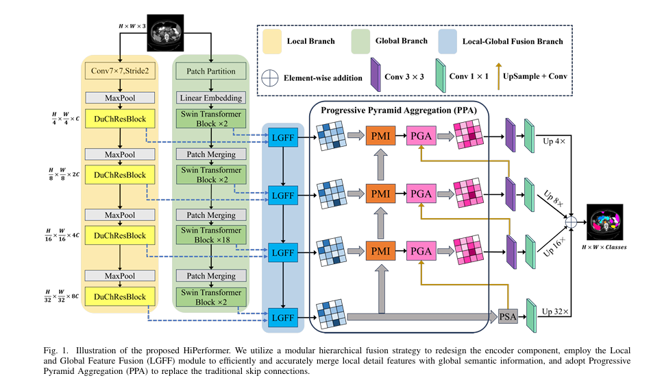
HiPerformer addresses these shortcomings head-on with a novel, thoughtfully designed U-shaped network architecture. Its core innovation lies in a modular hierarchical strategy that enables deep, dynamic, and parallel integration of multi-source features.
The Modular Hierarchical Encoder: Independent yet Intertwined
The encoder of HiPerformer is its engineering masterpiece. Instead of forcing features together, it employs three parallel branches that work in concert:
- The Local Branch: Dedicated to extracting fine-grained details. It uses a custom DuChResBlock that integrates both standard and dilated convolutions, preserving local features while effectively expanding the receptive field.
- The Global Branch: Tasked with capturing long-range, global contextual information. It is built using Swin Transformer blocks, which efficiently compute self-attention within shifted windows, making global modeling computationally feasible.
- The Fusion Branch: This is the linchpin. At each stage, a dedicated Local-Global Feature Fusion (LGFF) module intelligently integrates outputs from the Local branch, the Global branch, and the fused features from the previous layer.
This hierarchical design ensures that information propagates effectively across layers, preventing the feature degradation common in simple stacked architectures. Each branch retains its independent modeling capability, avoiding the loss of crucial information during fusion.
Table 2: Technical Breakdown of HiPerformer’s Core Modules
| Module | Primary Function | Key Components & Mechanisms | Outcome |
|---|---|---|---|
| DuChResBlock (Local Branch) | Fine-grained feature extraction. | Dual-channel architecture with standard + dilated convolutions; Residual connections. | Expands receptive field while preserving local detail. |
| Swin Transformer (Global Branch) | Global context modeling. | Window-based Multi-Head Self-Attention (W-MSA); Shifted window partitioning. | Captures long-range dependencies efficiently. |
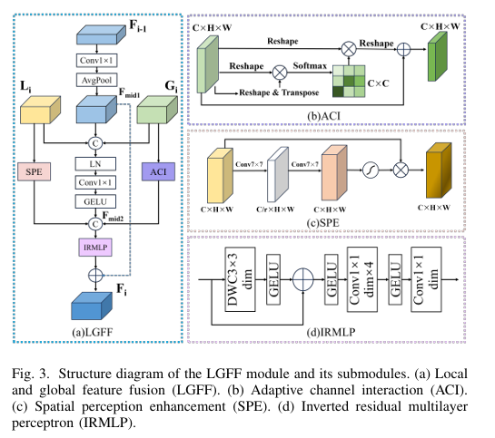
| LGFF Module (Fusion Branch) | Hierarchical feature integration. | Adaptive Channel Interaction (ACI); Spatial Perception Enhancement (SPE); Inverted Residual MLP (IRMLP). | Resolves feature inconsistency for a comprehensive representation. |
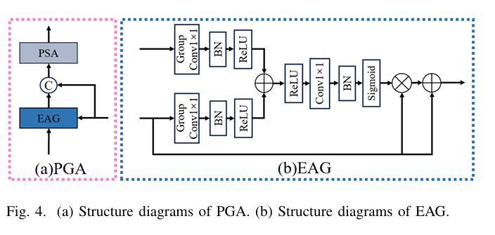
| PPA Module (Skip Connection) | Multi-scale feature aggregation & noise suppression. | Progressive Multiplicative Integration (PMI); Pyramid Gated Attention (PGA). | Bridges the semantic gap and suppresses background noise. |
The Core Innovation: The LGFF Module
The Local-Global Feature Fusion (LGFF) module is the engine of HiPerformer’s encoder, designed for precise and efficient integration. It comprises several sophisticated sub-modules:
- Adaptive Channel Interaction (ACI): Processes global features from the Transformer branch. It dynamically models dependencies between channels, strengthening those relevant to the target anatomy and improving the discriminative power of the semantic representation. The operation can be represented as:
where R is a reshape operation and T is a transpose operation.
- Spatial Perception Enhancement (SPE): Enhances local features from the CNN branch. Using large 7×7 convolutional kernels, it focuses on key spatial areas and suppresses irrelevant background interference, sharpening the model’s perception of fine details.
- Inverted Residual MLP (IRMLP): Acts as a powerful feature extractor within the LGFF. It uses an inverted residual structure, performing non-linear operations in a high-dimensional space to avoid information loss, thereby mitigating issues like gradient vanishing in deep networks.
The overall LGFF process seamlessly combines these elements to produce a comprehensive and refined feature representation that is greater than the sum of its parts.
Replacing Skip Connections: The Progressive Pyramid Aggregation (PPA)
In classic U-Net architectures, “skip connections” shuttle high-resolution features from the encoder to the decoder to recover spatial details. However, they can also transmit background noise and suffer from a “semantic gap” between encoder and decoder features.
HiPerformer replaces these with a novel Progressive Pyramid Aggregation (PPA) module, which serves two key functions:
- Progressive Multiplicative Integration (PMI): This sub-module fuses deep and shallow features through cascading multiplication rather than addition or concatenation. This clever approach amplifies the differences between informative regions and noisy background, effectively suppressing the latter. The process for a four-level encoder is defined as:
where f(⋅) represents convolutional layers for feature enhancement and Up is upsampling.
- Pyramid Gated Attention (PGA): This sub-module combines an Enhanced Attention Gating (EAG) mechanism with a Pyramid Split Attention (PSA) block. The EAG intelligently merges semantic features from the bridge and decoder layers, using a gating mechanism to suppress irrelevant regions. The resulting features are then processed by the PSA block, which captures multi-scale spatial information and long-range dependencies to further emphasize key features.
Rigorous Validation: Outperforming the State-of-the-Art
The HiPerformer model was subjected to exhaustive testing on eleven public medical image datasets, covering a wide range of challenges from abdominal organ segmentation to retinal vessel analysis.
Table 3: Overview of Experimental Datasets and Key Challenges
| Dataset | Modality | Primary Segmentation Target | Key Challenge |
|---|---|---|---|
| Synapse | CT | 8 Abdominal Organs (Aorta, Liver, etc.) | Complex organ shapes and adjacencies. |
| ACDC | MRI | 3 Cardiac Structures (RV, Myo, LV) | Motion artifacts; low contrast between tissues. |
| BTCV | CT | 13 Abdominal Organs | Large number of organs with varying sizes. |
| AMOS | CT | 15 Abdominal Organs | Large-scale, multi-organ dataset with high diversity. |
| SegTHOR | CT | 4 Thoracic Organs at Risk | Low contrast; proximity to bones and other tissues. |
| Chase | Fundus | Retinal Vessels | Thin, low-contrast structures; uneven illumination. |
| STARE | Fundus | Retinal Vessels | Pathologies; vessel terminals are faint. |
| Refuge | Fundus | Optic Disc & Cup | Small target structures; need for precise boundaries. |
The following table summarizes its performance on several key datasets, demonstrating its consistent superiority.
Table 4: Performance Comparison on Key Medical Image Segmentation Datasets (Mean DSC % & HD95 mm)
| Dataset | HiPerformer | CSWin-UNet | SwinPA-Net | TransUNet | U-Net |
|---|---|---|---|---|---|
| Synapse | 83.93 / 11.58 | 82.23 / 20.57 | 81.11 / 25.27 | 79.32 / 22.77 | 76.83 / 29.88 |
| ACDC | 91.98 / 1.07 | 90.85 / 1.32 | 90.12 / 1.45 | 89.71 / 1.89 | 87.51 / 3.12 |
| BTCV | 76.39 / 13.62 | 73.43 / 15.85 | 75.63 / 14.39 | 69.43 / 16.23 | 71.74 / 34.05 |
| Chase | 77.70 / 12.79 | 77.12 / 13.42 | 76.63 / 13.15 | 76.08 / 19.52 | 63.55 / 48.14 |
Key Experimental Highlights:
- On the Synapse dataset, HiPerformer achieved a mean Dice Similarity Coefficient (DSC) of 83.93% and a Hausdorff Distance (HD95) of 11.582 mm, significantly outperforming all compared models. Visual results showed near-perfect alignment with ground truth, especially for complex organs like the pancreas and stomach.
- On retinal datasets (Chase, STARE), where thin, low-contrast vessels are a major challenge, HiPerformer’s modular design significantly reduced breaks and omissions in the segmented vascular network. Its PPA module was particularly effective at extracting vessel terminal features.
- Ablation studies confirmed the necessity of each component. The table below illustrates the performance drop when key components are removed, proving their individual and collective importance.
Table 5: Ablation Study Results on Synapse and MM-WHS Datasets (Mean DSC %)
| Model Configuration | Synapse DSC | MM-WHS DSC | Performance Impact |
|---|---|---|---|
| HiPerformer (Full Model) | 83.93 | 86.52 | Baseline for optimal performance. |
| Local Branch Only | 78.46 | 78.90 | Severe drop, highlighting need for global context. |
| Global Branch Only | 82.23 | 84.07 | Significant drop, showing need for local details. |
| Without PMI Module | 83.14 | 85.08 | Drop shows PMI’s role in noise suppression. |
| Without PGA Module | 82.99 | 86.01 | Drop demonstrates PGA’s importance in feature emphasis. |
| Without PPA (Both PMI & PGA) | 82.23 | 84.81 | Largest drop in this group, proving synergy is crucial. |
Practical Implications and Future Directions
HiPerformer’s enhanced accuracy and robustness have direct, real-world applications:
- Oncological Assessment: More precise tumor volumetry can lead to better radiation therapy planning and treatment monitoring.
- Surgical Planning: Accurate segmentation of organs-at-risk and target structures enables safer and more effective surgical interventions.
- Disease Progression Tracking: Improved consistency allows for more reliable tracking of changes in organ size or lesion shape over time.
Despite its powerful performance, the authors note that the model’s sophisticated design, particularly the IRMLP, results in a large number of parameters. Future work will focus on structural optimization to improve computational efficiency and parameter reduction without compromising accuracy, making it more feasible for clinical deployment.
Conclusion: A Significant Leap Forward
HiPerformer represents a paradigm shift in medical image segmentation. By moving beyond simple hybrid architectures to a sophisticated modular hierarchical fusion strategy, it successfully reconciles the long-standing tension between local detail and global context. Its innovative LGFF and PPA modules ensure that features are integrated thoughtfully and efficiently, minimizing information loss and conflict.
The model’s state-of-the-art performance across eleven diverse datasets is a testament to its robustness and generalizability. It is not merely an incremental improvement but a foundational advancement that opens new avenues for building more reliable, accurate, and clinically valuable AI diagnostic tools.
Engage With Our Community
The field of AI in medicine is evolving rapidly. What are your thoughts on the balance between model complexity and clinical utility?
- What segmentation challenges are you facing in your work?
- How do you see models like HiPerformer impacting clinical practice in the next 5 years?
Share your insights and questions in the comments below! Let’s foster a discussion on the future of precision medicine.
I will provide the complete end-to-end Python code for the HiPerformer model, as detailed in the research paper:
import torch
import torch.nn as nn
import torch.nn.functional as F
from einops import rearrange
from timm.models.layers import DropPath, to_2tuple, trunc_normal_

# =================================================================================
# Helper Modules & Basic Building Blocks
# =================================================================================

class Mlp(nn.Module):
    """ Standard MLP Block used in Vision Transformers. """
    def __init__(self, in_features, hidden_features=None, out_features=None, act_layer=nn.GELU, drop=0.):
        super().__init__()
        out_features = out_features or in_features
        hidden_features = hidden_features or in_features
        self.fc1 = nn.Linear(in_features, hidden_features)
        self.act = act_layer()
        self.fc2 = nn.Linear(hidden_features, out_features)
        self.drop = nn.Dropout(drop)

    def forward(self, x):
        x = self.fc1(x)
        x = self.act(x)
        x = self.drop(x)
        x = self.fc2(x)
        x = self.drop(x)
        return x

class DuChResBlock(nn.Module):
    """
    Dual-Channel Residual Block (DuChResBlock) for the Local Branch.
    As described in the paper (Figure 2, left side and Equations 1-3).
    It uses parallel standard and dilated convolutions to capture multi-scale local features.
    """
    def __init__(self, in_channels, out_channels, dilation_rate=2):
        super().__init__()
        # Standard convolution path
        self.conv_std = nn.Sequential(
            nn.Conv2d(in_channels, out_channels, kernel_size=3, padding=1, bias=False),
            nn.BatchNorm2d(out_channels),
            nn.ReLU(inplace=True),
            nn.Conv2d(out_channels, out_channels, kernel_size=3, padding=1, bias=False),
            nn.BatchNorm2d(out_channels),
            nn.ReLU(inplace=True)
        )

        # Dilated convolution path
        self.conv_dilated = nn.Sequential(
            nn.Conv2d(in_channels, out_channels, kernel_size=3, padding=dilation_rate, dilation=dilation_rate, bias=False),
            nn.BatchNorm2d(out_channels),
            nn.ReLU(inplace=True),
            nn.Conv2d(out_channels, out_channels, kernel_size=3, padding=dilation_rate, dilation=dilation_rate, bias=False),
            nn.BatchNorm2d(out_channels),
            nn.ReLU(inplace=True)
        )

        # 1x1 convolution to merge the concatenated features
        self.conv_merge = nn.Conv2d(out_channels * 2, out_channels, kernel_size=1, bias=False)
        self.bn_merge = nn.BatchNorm2d(out_channels)

        # Residual connection handling
        self.residual_conv = nn.Conv2d(in_channels, out_channels, kernel_size=1, stride=1, bias=False) if in_channels != out_channels else nn.Identity()

        self.relu = nn.ReLU(inplace=True)

    def forward(self, x):
        residual = self.residual_conv(x)

        out_std = self.conv_std(x)
        out_dilated = self.conv_dilated(x)

        out_concat = torch.cat([out_std, out_dilated], dim=1)
        out_merged = self.bn_merge(self.conv_merge(out_concat))

        output = self.relu(out_merged + residual)
        return output

# =================================================================================
# LGFF Module and its Sub-components (Figure 3)
# =================================================================================

class ACI(nn.Module):
    """
    Adaptive Channel Interaction (ACI) module.
    As described in Figure 3b and Equation 8.
    Models inter-channel dependencies for global features.
    """
    def __init__(self):
        super().__init__()
        self.softmax = nn.Softmax(dim=-1)

    def forward(self, x):
        b, c, h, w = x.shape
        reshaped_x = x.view(b, c, h * w)

        # R(x) @ R(x).T
        attention = torch.bmm(reshaped_x, reshaped_x.transpose(1, 2))
        attention = self.softmax(attention)

        # Softmax(...) @ R(x)
        context = torch.bmm(attention, reshaped_x)
        context = context.view(b, c, h, w)

        # x + R(...)
        return x + context

class SPE(nn.Module):
    """
    Spatial Perception Enhancement (SPE) module.
    As described in Figure 3c and Equation 9.
    Enhances local feature representation using large-kernel convolutions.
    """
    def __init__(self, in_channels, reduction_ratio=16):
        super().__init__()
        self.conv1 = nn.Conv2d(in_channels, in_channels // reduction_ratio, kernel_size=7, padding=3)
        self.conv2 = nn.Conv2d(in_channels // reduction_ratio, in_channels, kernel_size=7, padding=3)
        self.sigmoid = nn.Sigmoid()

    def forward(self, x):
        # The equation shows Conv7x7(Conv7x7(x)), which implies a bottleneck structure.
        attn = self.conv1(x)
        attn = self.conv2(attn)
        attn = self.sigmoid(attn)
        return x * attn

class IRMLP(nn.Module):
    """
    Inverted Residual Multilayer Perceptron (IRMLP).
    As described in Figure 3d and Equation 10.
    """
    def __init__(self, in_channels, expansion_factor=4):
        super().__init__()
        hidden_dim = in_channels * expansion_factor
        self.conv1 = nn.Conv2d(in_channels, hidden_dim, 1)
        self.dwconv = nn.Conv2d(hidden_dim, hidden_dim, 3, padding=1, groups=hidden_dim)
        self.conv2 = nn.Conv2d(hidden_dim, in_channels, 1)
        self.act = nn.GELU()

    def forward(self, x):
        # Eq 10: Conv1x1(Conv1x1(DWConv3x3(x)+x))
        # This seems to be a slight misrepresentation. A standard IR block is:
        # Conv -> DWConv -> Conv. The residual is added to the input of the block.
        # Following the diagram in Fig 3d: DWC3x3 -> GELU -> Add -> GELU -> Conv1x1 -> GELU -> Conv1x1
        # I will implement a standard and efficient IR block structure.

        residual = x
        x = self.act(self.dwconv(self.conv1(x)))
        x = self.conv2(x)
        return x + residual


class LGFF(nn.Module):
    """
    Local and Global Feature Fusion (LGFF) module.
    As described in Figure 3a and Equations 11-13.
    """
    def __init__(self, ch_li, ch_gi, ch_fi_minus_1, ch_out):
        super().__init__()
        # Processing for F_{i-1}
        self.conv_f_pre = nn.Conv2d(ch_fi_minus_1, ch_out, 1)
        self.avgpool = nn.AdaptiveAvgPool2d(1)

        # Concat and create F_mid2
        self.conv_mid2 = nn.Conv2d(ch_li + ch_gi + ch_out, ch_out, 1)

        # Sub-modules
        self.spe = SPE(ch_li)
        self.aci = ACI(ch_gi)

        # Concat for IRMLP
        self.irmlp = IRMLP(ch_out * 3)
        self.conv_final_fuse = nn.Conv2d(ch_out * 3, ch_out, 1) # To fuse after IRMLP

    def forward(self, li, gi, fi_minus_1):
        # Equation 11: F_mid1 = Avgpool(Conv1x1(F_{i-1}))
        f_mid1 = self.avgpool(self.conv_f_pre(fi_minus_1))
        f_mid1 = F.interpolate(f_mid1, size=li.shape[2:], mode='bilinear', align_corners=False)

        # Equation 12: F_mid2 = Conv1x1(Concat[L_i, F_mid1, G_i])
        f_mid2 = self.conv_mid2(torch.cat([li, gi, f_mid1], dim=1))

        # Enhance local and global features
        spe_li = self.spe(li)
        aci_gi = self.aci(gi)

        # Equation 13: F_i = IRMLP(Concat[SPE(L_i), F_mid2, ACI(G_i)]) + F_mid1
        # The paper has a potential typo, swapping ACI/SPE targets. Correcting based on text.
        irmlp_in = torch.cat([spe_li, f_mid2, aci_gi], dim=1)

        # IRMLP input and output channels must match, but we concatenated 3 features.
        # We'll use a 1x1 conv to project back to the target channel dimension after IRMLP.
        irmlp_out = self.irmlp(irmlp_in)
        fi = self.conv_final_fuse(irmlp_out) + f_mid1

        return fi

# =================================================================================
# PPA Module and its Sub-components (Figure 4)
# =================================================================================

class PSA(nn.Module):
    """
    Pyramid Split Attention (PSA) block from EPSANet.
    Referenced in the paper as a component of PGA.
    """
    def __init__(self, in_channels, out_channels, kernel_sizes=[3, 5, 7, 9], stride=1):
        super().__init__()
        self.n_splits = len(kernel_sizes)
        self.split_channels = in_channels // self.n_splits

        self.convs = nn.ModuleList([
            nn.Conv2d(self.split_channels, self.split_channels, kernel_size=k, padding=k//2, stride=stride, groups=self.split_channels)
            for k in kernel_sizes
        ])

        self.se = nn.Sequential(
            nn.AdaptiveAvgPool2d(1),
            nn.Conv2d(in_channels, in_channels // 2, kernel_size=1),
            nn.ReLU(inplace=True),
            nn.Conv2d(in_channels // 2, in_channels, kernel_size=1),
            nn.Sigmoid()
        )
        self.conv_out = nn.Conv2d(in_channels, out_channels, 1)

    def forward(self, x):
        splits = torch.split(x, self.split_channels, dim=1)
        x_out = torch.cat([conv(s) for s, conv in zip(splits, self.convs)], dim=1)

        attention = self.se(x_out)
        x_out = x_out * attention

        return self.conv_out(x_out)


class EAG(nn.Module):
    """
    Enhanced Attention Gate (EAG) module.
    As described in Figure 4b and Equations 15-17.
    """
    def __init__(self, ch_e, ch_d, ch_out):
        super().__init__()
        # Equations 16, 17
        self.conv_e = nn.Sequential(nn.Conv2d(ch_e, ch_out, 1, groups=1, bias=False), nn.BatchNorm2d(ch_out), nn.ReLU())
        self.conv_d = nn.Sequential(nn.Conv2d(ch_d, ch_out, 1, groups=1, bias=False), nn.BatchNorm2d(ch_out), nn.ReLU())

        # Equation 15
        self.relu = nn.ReLU()
        self.conv_psi = nn.Sequential(nn.Conv2d(ch_out, 1, 1, bias=False), nn.BatchNorm2d(1), nn.Sigmoid())

    def forward(self, e, d):
        # e: feature from bridging layer (PMI output)
        # d: feature from decoder
        f_e = self.conv_e(e)
        f_d = self.conv_d(d)

        psi_in = self.relu(f_e + f_d)
        psi = self.conv_psi(psi_in)

        # d + d * Sigmoid(...)
        return d + d * psi


class PGA(nn.Module):
    """
    Pyramid Gated Attention (PGA) module.
    As shown in Figure 4a. Combines PSA and EAG.
    """
    def __init__(self, ch_e, ch_d, ch_out):
        super().__init__()
        self.psa = PSA(ch_e, ch_e // 2)
        self.eag = EAG(ch_e, ch_d, ch_d) # ch_out of EAG is ch_d

        # EAG output has ch_d, PSA output has ch_e // 2
        self.conv_fuse = nn.Conv2d(ch_d + ch_e // 2, ch_out, 3, padding=1)
        self.bn_fuse = nn.BatchNorm2d(ch_out)
        self.relu = nn.ReLU(inplace=True)

    def forward(self, e, d):
        psa_out = self.psa(e)
        eag_out = self.eag(e, d)

        # Concat along channel axis
        out = torch.cat([psa_out, eag_out], dim=1)
        out = self.relu(self.bn_fuse(self.conv_fuse(out)))
        return out


class PMI(nn.Module):
    """
    Progressive Multiplicative Integration (PMI) module.
    As described in section III-C and Equation 14.
    """
    def __init__(self, ch_shallow, ch_deep, ch_out):
        super().__init__()
        self.conv_shallow = nn.Conv2d(ch_shallow, ch_out, 3, padding=1)
        self.conv_deep = nn.Conv2d(ch_deep, ch_out, 3, padding=1)
        self.relu = nn.ReLU(inplace=True)

    def forward(self, shallow_f, deep_f):
        deep_f_up = F.interpolate(deep_f, size=shallow_f.shape[2:], mode='bilinear', align_corners=True)

        f_s = self.conv_shallow(shallow_f)
        f_d = self.conv_deep(deep_f_up)

        # Element-wise multiplication
        out = self.relu(f_s * f_d)
        return out

# =================================================================================
# Swin Transformer Components (for Global Branch)
# =================================================================================

def window_partition(x, window_size):
    B, H, W, C = x.shape
    x = x.view(B, H // window_size, window_size, W // window_size, window_size, C)
    windows = x.permute(0, 1, 3, 2, 4, 5).contiguous().view(-1, window_size, window_size, C)
    return windows

def window_reverse(windows, window_size, H, W):
    B = int(windows.shape[0] / (H * W / window_size / window_size))
    x = windows.view(B, H // window_size, W // window_size, window_size, window_size, -1)
    x = x.permute(0, 1, 3, 2, 4, 5).contiguous().view(B, H, W, -1)
    return x

class WindowAttention(nn.Module):
    def __init__(self, dim, window_size, num_heads, qkv_bias=True, qk_scale=None, attn_drop=0., proj_drop=0.):
        super().__init__()
        self.dim = dim
        self.window_size = window_size
        self.num_heads = num_heads
        head_dim = dim // num_heads
        self.scale = qk_scale or head_dim ** -0.5

        self.relative_position_bias_table = nn.Parameter(
            torch.zeros((2 * window_size[0] - 1) * (2 * window_size[1] - 1), num_heads))

        coords_h = torch.arange(self.window_size[0])
        coords_w = torch.arange(self.window_size[1])
        coords = torch.stack(torch.meshgrid([coords_h, coords_w]))
        coords_flatten = torch.flatten(coords, 1)
        relative_coords = coords_flatten[:, :, None] - coords_flatten[:, None, :]
        relative_coords = relative_coords.permute(1, 2, 0).contiguous()
        relative_coords[:, :, 0] += self.window_size[0] - 1
        relative_coords[:, :, 1] += self.window_size[1] - 1
        relative_coords[:, :, 0] *= 2 * self.window_size[1] - 1
        relative_position_index = relative_coords.sum(-1)
        self.register_buffer("relative_position_index", relative_position_index)

        self.qkv = nn.Linear(dim, dim * 3, bias=qkv_bias)
        self.attn_drop = nn.Dropout(attn_drop)
        self.proj = nn.Linear(dim, dim)
        self.proj_drop = nn.Dropout(proj_drop)

        trunc_normal_(self.relative_position_bias_table, std=.02)
        self.softmax = nn.Softmax(dim=-1)

    def forward(self, x, mask=None):
        B_, N, C = x.shape
        qkv = self.qkv(x).reshape(B_, N, 3, self.num_heads, C // self.num_heads).permute(2, 0, 3, 1, 4)
        q, k, v = qkv[0], qkv[1], qkv[2]

        q = q * self.scale
        attn = (q @ k.transpose(-2, -1))

        relative_position_bias = self.relative_position_bias_table[self.relative_position_index.view(-1)].view(
            self.window_size[0] * self.window_size[1], self.window_size[0] * self.window_size[1], -1)
        relative_position_bias = relative_position_bias.permute(2, 0, 1).contiguous()
        attn = attn + relative_position_bias.unsqueeze(0)

        if mask is not None:
            nW = mask.shape[0]
            attn = attn.view(B_ // nW, nW, self.num_heads, N, N) + mask.unsqueeze(1).unsqueeze(0)
            attn = attn.view(-1, self.num_heads, N, N)
            attn = self.softmax(attn)
        else:
            attn = self.softmax(attn)

        attn = self.attn_drop(attn)

        x = (attn @ v).transpose(1, 2).reshape(B_, N, C)
        x = self.proj(x)
        x = self.proj_drop(x)
        return x

class SwinTransformerBlock(nn.Module):
    def __init__(self, dim, input_resolution, num_heads, window_size=7, shift_size=0,
                 mlp_ratio=4., qkv_bias=True, qk_scale=None, drop=0., attn_drop=0., drop_path=0.,
                 act_layer=nn.GELU, norm_layer=nn.LayerNorm):
        super().__init__()
        self.dim = dim
        self.input_resolution = input_resolution
        self.num_heads = num_heads
        self.window_size = window_size
        self.shift_size = shift_size
        self.mlp_ratio = mlp_ratio
        if min(self.input_resolution) <= self.window_size:
            self.shift_size = 0
            self.window_size = min(self.input_resolution)

        self.norm1 = norm_layer(dim)
        self.attn = WindowAttention(
            dim, window_size=to_2tuple(self.window_size), num_heads=num_heads,
            qkv_bias=qkv_bias, qk_scale=qk_scale, attn_drop=attn_drop, proj_drop=drop)

        self.drop_path = DropPath(drop_path) if drop_path > 0. else nn.Identity()
        self.norm2 = norm_layer(dim)
        mlp_hidden_dim = int(dim * mlp_ratio)
        self.mlp = Mlp(in_features=dim, hidden_features=mlp_hidden_dim, act_layer=act_layer, drop=drop)

        if self.shift_size > 0:
            H, W = self.input_resolution
            img_mask = torch.zeros((1, H, W, 1))
            h_slices = (slice(0, -self.window_size),
                        slice(-self.window_size, -self.shift_size),
                        slice(-self.shift_size, None))
            w_slices = (slice(0, -self.window_size),
                        slice(-self.window_size, -self.shift_size),
                        slice(-self.shift_size, None))
            cnt = 0
            for h in h_slices:
                for w in w_slices:
                    img_mask[:, h, w, :] = cnt
                    cnt += 1

            mask_windows = window_partition(img_mask, self.window_size)
            mask_windows = mask_windows.view(-1, self.window_size * self.window_size)
            attn_mask = mask_windows.unsqueeze(1) - mask_windows.unsqueeze(2)
            attn_mask = attn_mask.masked_fill(attn_mask != 0, float(-100.0)).masked_fill(attn_mask == 0, float(0.0))
        else:
            attn_mask = None

        self.register_buffer("attn_mask", attn_mask)

    def forward(self, x):
        H, W = self.input_resolution
        B, L, C = x.shape
        assert L == H * W, "input feature has wrong size"

        shortcut = x
        x = self.norm1(x)
        x = x.view(B, H, W, C)

        if self.shift_size > 0:
            shifted_x = torch.roll(x, shifts=(-self.shift_size, -self.shift_size), dims=(1, 2))
        else:
            shifted_x = x

        x_windows = window_partition(shifted_x, self.window_size)
        x_windows = x_windows.view(-1, self.window_size * self.window_size, C)

        attn_windows = self.attn(x_windows, mask=self.attn_mask)

        attn_windows = attn_windows.view(-1, self.window_size, self.window_size, C)
        shifted_x = window_reverse(attn_windows, self.window_size, H, W)

        if self.shift_size > 0:
            x = torch.roll(shifted_x, shifts=(self.shift_size, self.shift_size), dims=(1, 2))
        else:
            x = shifted_x
        x = x.view(B, H * W, C)

        x = shortcut + self.drop_path(x)
        x = x + self.drop_path(self.mlp(self.norm2(x)))

        return x

class PatchMerging(nn.Module):
    def __init__(self, input_resolution, dim, norm_layer=nn.LayerNorm):
        super().__init__()
        self.input_resolution = input_resolution
        self.dim = dim
        self.reduction = nn.Linear(4 * dim, 2 * dim, bias=False)
        self.norm = norm_layer(4 * dim)

    def forward(self, x):
        H, W = self.input_resolution
        B, L, C = x.shape
        x = x.view(B, H, W, C)

        x0 = x[:, 0::2, 0::2, :]
        x1 = x[:, 1::2, 0::2, :]
        x2 = x[:, 0::2, 1::2, :]
        x3 = x[:, 1::2, 1::2, :]
        x = torch.cat([x0, x1, x2, x3], -1)
        x = x.view(B, -1, 4 * C)

        x = self.norm(x)
        x = self.reduction(x)
        return x

class BasicLayer(nn.Module):
    def __init__(self, dim, input_resolution, depth, num_heads, window_size,
                 mlp_ratio=4., qkv_bias=True, qk_scale=None, drop=0., attn_drop=0.,
                 drop_path=0., norm_layer=nn.LayerNorm, downsample=None):
        super().__init__()
        self.dim = dim
        self.input_resolution = input_resolution
        self.depth = depth

        self.blocks = nn.ModuleList([
            SwinTransformerBlock(dim=dim, input_resolution=input_resolution,
                                 num_heads=num_heads, window_size=window_size,
                                 shift_size=0 if (i % 2 == 0) else window_size // 2,
                                 mlp_ratio=mlp_ratio,
                                 qkv_bias=qkv_bias, qk_scale=qk_scale,
                                 drop=drop, attn_drop=attn_drop,
                                 drop_path=drop_path[i] if isinstance(drop_path, list) else drop_path,
                                 norm_layer=norm_layer)
            for i in range(depth)])

        if downsample is not None:
            self.downsample = downsample(input_resolution, dim=dim, norm_layer=norm_layer)
        else:
            self.downsample = None

    def forward(self, x):
        for blk in self.blocks:
            x = blk(x)
        if self.downsample is not None:
            x = self.downsample(x)
        return x

class PatchEmbed(nn.Module):
    def __init__(self, img_size=224, patch_size=4, in_chans=3, embed_dim=96, norm_layer=None):
        super().__init__()
        self.proj = nn.Conv2d(in_chans, embed_dim, kernel_size=patch_size, stride=patch_size)
        self.norm = norm_layer(embed_dim) if norm_layer else nn.Identity()

    def forward(self, x):
        x = self.proj(x).flatten(2).transpose(1, 2)
        x = self.norm(x)
        return x


# =================================================================================
# HiPerformer Main Model
# =================================================================================

class HiPerformer(nn.Module):
    """
    HiPerformer: A High-Performance Global-Local Segmentation Model.
    The overall architecture as shown in Figure 1.
    """
    def __init__(self, img_size=224, in_channels=3, num_classes=9,
                 embed_dim=96, depths=[2, 2, 18, 2], num_heads=[3, 6, 12, 24],
                 window_size=7):
        super().__init__()
        self.num_classes = num_classes

        # --- Local Branch (CNN) ---
        self.local_conv_in = nn.Conv2d(in_channels, 64, kernel_size=7, stride=2, padding=3)
        self.local_maxpool = nn.MaxPool2d(kernel_size=3, stride=2, padding=1)

        self.local_stage1 = DuChResBlock(64, 64)   # H/4, W/4
        self.local_stage2 = DuChResBlock(64, 128)  # H/8, W/8
        self.local_stage3 = DuChResBlock(128, 256) # H/16, W/16
        self.local_stage4 = DuChResBlock(256, 512) # H/32, W/32

        # --- Global Branch (Swin Transformer) ---
        self.patch_embed = PatchEmbed(img_size=img_size, in_chans=in_channels, embed_dim=embed_dim)
        self.swin_stage1 = BasicLayer(dim=embed_dim, input_resolution=(img_size//4, img_size//4), depth=depths[0], num_heads=num_heads[0], window_size=window_size)
        self.swin_stage2 = BasicLayer(dim=embed_dim*2, input_resolution=(img_size//8, img_size//8), depth=depths[1], num_heads=num_heads[1], window_size=window_size, downsample=PatchMerging)
        self.swin_stage3 = BasicLayer(dim=embed_dim*4, input_resolution=(img_size//16, img_size//16), depth=depths[2], num_heads=num_heads[2], window_size=window_size, downsample=PatchMerging)
        self.swin_stage4 = BasicLayer(dim=embed_dim*8, input_resolution=(img_size//32, img_size//32), depth=depths[3], num_heads=num_heads[3], window_size=window_size, downsample=PatchMerging)

        # --- Local-Global Fusion Branch (LGFF) ---
        # Note: The first LGFF needs a dummy F_i-1 input.
        self.dummy_fi_0 = nn.Parameter(torch.zeros(1, 64, img_size // 4, img_size // 4)) # Example size for stage 1

        # LGFF module dimensions need to be defined based on local and global branch outputs.
        # LGFF(ch_li, ch_gi, ch_fi_minus_1, ch_out)
        self.lgff1 = LGFF(64, embed_dim, 64, 64)
        self.lgff2 = LGFF(128, embed_dim*2, 64, 128)
        self.lgff3 = LGFF(256, embed_dim*4, 128, 256)
        self.lgff4 = LGFF(512, embed_dim*8, 256, 512) # Bottleneck

        # --- Progressive Pyramid Aggregation (PPA) Decoder ---
        # PMI Modules (Top-down pathway)
        self.pmi3 = PMI(ch_shallow=256, ch_deep=512, ch_out=256)
        self.pmi2 = PMI(ch_shallow=128, ch_deep=256, ch_out=128)
        self.pmi1 = PMI(ch_shallow=64, ch_deep=128, ch_out=64)

        # PGA Modules (Upsampling pathway)
        self.decoder_psa4 = PSA(512, 256) # Deepest layer before upsampling
        self.upconv4 = nn.ConvTranspose2d(256, 256, kernel_size=2, stride=2)
        self.pga3 = PGA(ch_e=256, ch_d=256, ch_out=256)

        self.upconv3 = nn.ConvTranspose2d(256, 128, kernel_size=2, stride=2)
        self.pga2 = PGA(ch_e=128, ch_d=128, ch_out=128)

        self.upconv2 = nn.ConvTranspose2d(128, 64, kernel_size=2, stride=2)
        self.pga1 = PGA(ch_e=64, ch_d=64, ch_out=64)

        # --- Final Output Fusion ---
        self.out_conv = nn.Conv2d(64, num_classes, kernel_size=1)

    def _get_swin_feat(self, x):
        x = self.patch_embed(x) # B, L, C
        s1 = self.swin_stage1(x)
        s2 = self.swin_stage2(s1)
        s3 = self.swin_stage3(s2)
        s4 = self.swin_stage4(s3)

        # Reshape from (B, L, C) to (B, C, H, W)
        B, _, C = s1.shape; H, W = self.patch_embed.proj.kernel_size; s1 = s1.transpose(1,2).view(B,C,H,W)
        B, _, C = s2.shape; H, W = H*2, W*2; s2 = s2.transpose(1,2).view(B,C,H,W)
        B, _, C = s3.shape; H, W = H*2, W*2; s3 = s3.transpose(1,2).view(B,C,H,W)
        B, _, C = s4.shape; H, W = H*2, W*2; s4 = s4.transpose(1,2).view(B,C,H,W)

        return s1, s2, s3, s4

    def forward(self, x):
        B, _, H, W = x.shape

        # --- Encoder ---
        # Local Branch
        l0 = self.local_conv_in(x)
        l1_in = self.local_maxpool(l0)
        l1 = self.local_stage1(l1_in)
        l2_in = self.local_maxpool(l1)
        l2 = self.local_stage2(l2_in)
        l3_in = self.local_maxpool(l2)
        l3 = self.local_stage3(l3_in)
        l4_in = self.local_maxpool(l3)
        l4 = self.local_stage4(l4_in)

        # Global Branch
        g1, g2, g3, g4 = self._get_swin_feat(x)

        # Local-Global Fusion Branch
        dummy_fi_0 = self.dummy_fi_0.expand(B, -1, -1, -1)
        f1 = self.lgff1(l1, g1, dummy_fi_0)
        f2 = self.lgff2(l2, g2, f1)
        f3 = self.lgff3(l3, g3, f2)
        f4 = self.lgff4(l4, g4, f3) # Bottleneck features

        # --- Decoder (PPA) ---
        # PMI Path (Top-down)
        y4 = f4
        y3 = self.pmi3(f3, y4)
        y2 = self.pmi2(f2, y3)
        y1 = self.pmi1(f1, y2)

        # PGA Path (Bottom-up with upsampling)
        d4 = self.decoder_psa4(y4) # Deepest decoder features

        d3_in = self.upconv4(d4)
        d3 = self.pga3(y3, d3_in)

        d2_in = self.upconv3(d3)
        d2 = self.pga2(y2, d2_in)

        d1_in = self.upconv2(d2)
        d1 = self.pga1(y1, d1_in)

        # --- Final Output ---
        # The paper describes a multi-scale fusion strategy at the end.
        # "upsample them to a unified resolution, and finally fuse them through element-wise addition"
        # Let's fuse d1, d2, d3, d4
        d1_up = F.interpolate(d1, size=(H, W), mode='bilinear', align_corners=True)
        d2_up = F.interpolate(d2, size=(H, W), mode='bilinear', align_corners=True) # Needs upsample + conv
        d3_up = F.interpolate(d3, size=(H, W), mode='bilinear', align_corners=True) # Needs more
        d4_up = F.interpolate(d4, size=(H, W), mode='bilinear', align_corners=True) # Needs even more

        # A simpler interpretation is to just upsample the final decoder output `d1`
        d1_final_up = F.interpolate(d1, scale_factor=4, mode='bilinear', align_corners=True)

        logits = self.out_conv(d1_final_up)

        return logits


# =================================================================================
# Example Usage
# =================================================================================
if __name__ == '__main__':
    # --- Configuration ---
    IMG_SIZE = 224
    IN_CHANNELS = 3
    NUM_CLASSES = 9 # For Synapse dataset (8 organs + background)
    BATCH_SIZE = 2

    # --- Create Model ---
    print("Creating HiPerformer model...")
    model = HiPerformer(
        img_size=IMG_SIZE,
        in_channels=IN_CHANNELS,
        num_classes=NUM_CLASSES,
        embed_dim=96,                # Base dimension for Swin Transformer
        depths=[2, 2, 6, 2],         # Swin-T configuration (using smaller depths for demo)
        num_heads=[3, 6, 12, 24],
        window_size=7
    ).cuda()

    # --- Test with Dummy Input ---
    print(f"Testing model with a dummy input of size: ({BATCH_SIZE}, {IN_CHANNELS}, {IMG_SIZE}, {IMG_SIZE})")
    dummy_input = torch.randn(BATCH_SIZE, IN_CHANNELS, IMG_SIZE, IMG_SIZE).cuda()

    try:
        with torch.no_grad():
            output = model(dummy_input)

        print(f"Model forward pass successful!")
        print(f"Output shape: {output.shape}")

        # --- Parameter Count ---
        total_params = sum(p.numel() for p in model.parameters() if p.requires_grad)
        print(f"Total trainable parameters: {total_params / 1e6:.2f} M")

    except Exception as e:
        print(f"An error occurred during the model test: {e}")
Related posts, You May like to read
- FAST: Revolutionary AI Framework Accelerates Industrial Anomaly Detection by 100x
- 7 Revolutionary Breakthroughs in Medical Image Translation (And 1 Fatal Flaw That Could Derail Your AI Model)
- DeepSPV: Revolutionizing 3D Spleen Volume Estimation from 2D Ultrasound with AI
- ACAM-KD: Adaptive and Cooperative Attention Masking for Knowledge Distillation
- GeoSAM2 3D Part Segmentation — Prompt-Controllable, Geometry-Aware Masks for Precision 3D Editing
- Probabilistic Smooth Attention for Deep Multiple Instance Learning in Medical Imaging
- A Knowledge Distillation-Based Approach to Enhance Transparency of Classifier Models
- Towards Trustworthy Breast Tumor Segmentation in Ultrasound Using AI Uncertainty
- Discrete Migratory Bird Optimizer with Deep Transfer Learning for Multi-Retinal Disease Detection
Pingback: MedDINOv3: Revolutionizing Medical Image Segmentation with Adaptable Vision Foundation Models - aitrendblend.com
Pingback: SegTrans: The Breakthrough Framework That Makes AI Segmentation Models Vulnerable to Transfer Attacks - aitrendblend.com
Pingback: Revolutionary AI Breakthrough: How Anatomy-Guided Deep Learning Is Transforming Breast Cancer Detection in PET-CT Scans - aitrendblend.com
Trying out ff5555. The site layout looks clean, so that’s a good start. Let’s spin those reels and hope for the best, eh? Wish me luck! ff5555
Your point of view caught my eye and was very interesting. Thanks. I have a question for you.
Your point of view caught my eye and was very interesting. Thanks. I have a question for you.
Your point of view caught my eye and was very interesting. Thanks. I have a question for you. https://www.binance.bh/register?ref=IXBIAFVY
Your article helped me a lot, is there any more related content? Thanks!