HARP-NeXt: The Breakthrough LiDAR Segmentation Network That Delivers Real-Time Accuracy for Autonomous Vehicles

Introduction: Why Real-Time, Accurate LiDAR Segmentation is the Holy Grail for Self-Driving Cars

---

The LiDAR Segmentation Challenge: Speed vs. Accuracy on Embedded Systems

Before we dive into HARP-NeXt, let’s understand the landscape. Current LiDAR segmentation methods fall into four broad categories, each with distinct advantages and crippling drawbacks:

1. Point-Based Methods (e.g., PointNeXt, WaffleIron, PTv3)
   These operate directly on raw 3D points, preserving full geometric fidelity. They’re often the most accurate because they don’t lose information during projection. However, they rely heavily on computationally expensive operations like k-nearest neighbor (KNN) searches and farthest point sampling (FPS). On an NVIDIA Jetson AGX Orin—a common embedded platform for autonomous robots—PTv3 can take 872 milliseconds per scan. That’s nearly a second of processing time, far too slow for real-time navigation.
2. Projection-Based Methods (e.g., SalsaNext, CENet, FRNet)
   These project the 3D point cloud onto a 2D range image (like a spherical panorama), then use highly optimized 2D CNNs for segmentation. This approach is fast—SalsaNext runs in under 50ms on Jetson—but accuracy suffers. Critical spatial relationships get distorted or lost during projection, leading to misclassifications, especially around object boundaries or complex scenes.
3. Sparse Convolution-Based Methods (e.g., MinkowskiNet, Cylinder3D)
   These quantize points into sparse voxels and apply convolutions only where data exists, ignoring empty space. This reduces memory and computation compared to dense 3D convolutions. While accurate, they remain too slow for real-time use on embedded systems due to the complexity of managing sparse tensor operations.
4. Fusion-Based Methods (e.g., SPVCNN, RPVNet, 2DPASS)
   These combine multiple representations—say, 3D points and 2D images—to leverage the strengths of each. While promising, fusing data streams adds significant computational overhead, making them bulky and inefficient for mobile applications.

A recent study by Abou Haidar et al. [14] highlighted a crucial, often overlooked bottleneck: pre-processing. Converting raw LiDAR scans into a format suitable for neural networks involves CPU-bound tasks like spherical projection and coordinate mapping. On many systems, this phase can consume up to 83% of total execution time. Most state-of-the-art models ignore this, focusing solely on inference speed.

Key Takeaway: The quest for real-time LiDAR segmentation isn’t just about building a faster model; it’s about optimizing the entire pipeline, from raw data ingestion to final prediction.

---

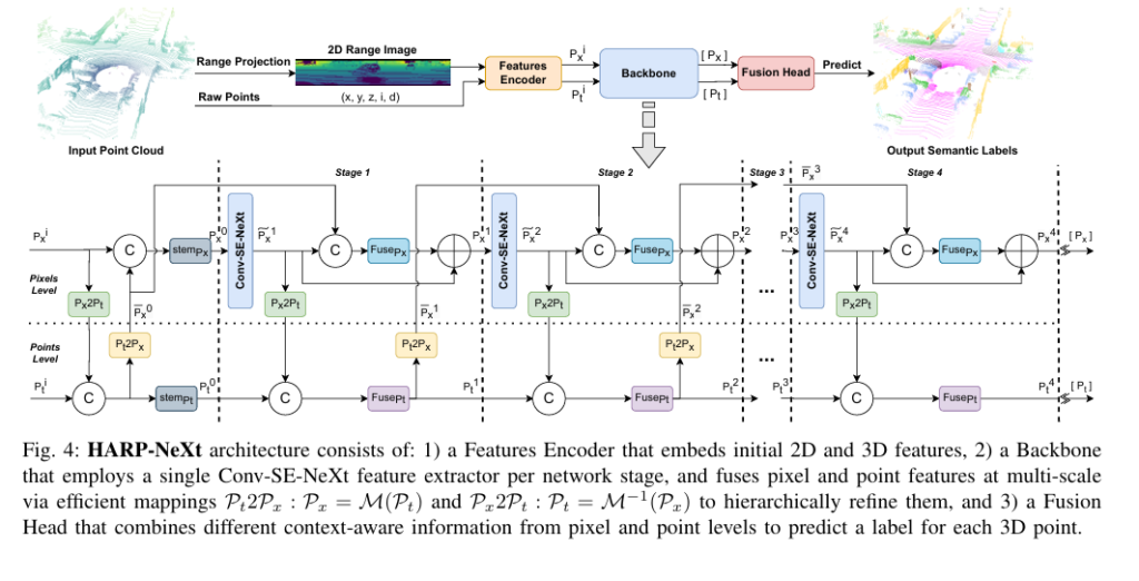
Introducing HARP-NeXt: Architecture, Innovations, and Core Components

HARP-NeXt stands for High-speed and Accurate Range-Point Fusion Network. Its brilliance lies not in inventing entirely new concepts, but in intelligently combining and optimizing existing ones to achieve unprecedented efficiency without sacrificing accuracy.

The network’s core philosophy is multi-scale range-point fusion. Instead of treating 2D pixels and 3D points as separate entities, HARP-NeXt creates a seamless bridge between them, allowing features to be exchanged and refined across different levels of abstraction. Think of it as a collaborative system where 2D vision provides context and 3D geometry provides precision.

Here’s a breakdown of its key architectural components:

1. GPU-Accelerated Preprocessing: Turning Bottlenecks into Advantages

This is perhaps HARP-NeXt’s most underrated innovation. Traditional workflows load raw data into CPU memory, preprocess it entirely on the CPU (converting coordinates, projecting to range images, clustering points), collate the data, and then transfer it to the GPU for inference. This process is serial, CPU-intensive, and creates a massive data transfer bottleneck.

HARP-NeXt flips this script:

Classical Workflow:
Load Raw Data → CPU Preprocess → Collate → Move to GPU → Inference

HARP-NeXt Workflow:
Load Raw Data → Collate Raw → IMMEDIATE Move to GPU → GPU Preprocess → Inference

By moving raw data to the GPU first, HARP-NeXt leverages the GPU’s parallel processing power for tasks like spherical projection and feature extraction. This drastically reduces CPU load and minimizes data transfer latency. The result? Pre-processing time drops from hundreds of milliseconds to just 3–10 ms on high-end GPUs and 10–23 ms on Jetson Orin, making it the fastest pre-processing pipeline among all compared methods.

2. The Conv-SE-NeXt Block: Efficiency Meets Expressiveness

At the heart of HARP-NeXt’s backbone is the Conv-SE-NeXt block, a novel feature extraction module designed for maximum efficiency. It draws inspiration from ResNet, ConvNeXt, and SE-ResNet blocks but optimizes them for real-time performance.

The block uses depth-wise separable convolutions, which decompose a standard convolution into two steps:

• Depth-wise convolution (DWConv): Applies a single filter per input channel, capturing spatial patterns.
• Point-wise convolution (PWConv): Uses 1×1 convolutions to combine channels, aggregating features.

This decomposition reduces the number of parameters and computations significantly. For example, a standard 3×3 convolution on 64 input and 64 output channels requires 64×64×9=36,864 multiplications. A depth-wise separable version requires only 64×9+64×64=4,672 multiplications—a reduction of over 87%.

To further enhance feature learning, the block integrates a Squeeze-and-Excitation (SE) module. Unlike the original SE block that uses fully connected layers, HARP-NeXt employs 1×1 channel-wise convolutions for greater efficiency. The SE module calculates an attention weight for each channel based on global average pooling, allowing the network to focus on the most informative features.

The mathematical flow within the Conv-SE-NeXt block is as follows:

\[ \textbf{Depth-wise Convolution \& Activation:} \quad y_{dw} = \sigma\big(N(W_{dw} * x)\big) \] where Wdw is the depth-wise kernel, N denotes Batch Normalization, and σ is the Hardswish activation function (chosen for its efficiency and smooth nonlinearity). \[ \textbf{Point-wise Convolution:} \quad y_{pw} = N(W_{pw} * y_{dw}) \] where ypw is the point-wise kernel. \[ \textbf{Squeeze-and-Excitation:} \] **Global Average Pooling:** \[ z_{c} = \text{GAP}(y_{pw}) = \frac{1}{H \times W} \sum_{i=1}^{H} \sum_{j=1}^{W} y_{pw}(i,j) \] **Channel Attention:** \[ s_{c} = \sigma_{2}\big(W_{2} \, \sigma_{1}(W_{1} z_{c})\big) \] where σ1 is ReLU and σ2 is Hardsigmoid (a more efficient variant of Sigmoid). \[ \textbf{Feature Weighting:} \quad \tilde{y}_{c} = y_{pw} \odot s_{c} \] \[ \textbf{Residual Connection:} \quad z = \tilde{y}_{c} + x \] This residual path helps mitigate vanishing gradients and stabilizes training.

Key Takeaway: The Conv-SE-NeXt block is a powerhouse of efficiency. It captures rich spatial and channel-wise features with minimal computational cost, enabling HARP-NeXt to use only one such block per network stage instead of stacking multiple layers.

3. Multi-Scale Range-Point Fusion Backbone: Bridging the 2D-3D Divide

The backbone consists of four stages, each designed to fuse features from pixel (2D) and point (3D) levels hierarchically. The magic happens through efficient mapping functions:

• Pt2Px: Maps point features to pixel features (P_t​ → P_x​ ).
• Px2Pt: Maps pixel features back to point features (P_x​ → P_t​ ).

These mappings allow information to flow bidirectionally. At each stage, pixel features extracted by Conv-SE-NeXt are fused with mapped point features from the previous stage using bilinear interpolation and convolution. An attention mechanism then weights the fused features before refining the pixel representation in a residual manner.

Similarly, point features are refined by combining mapped pixel features with their own previous-stage features. This iterative refinement across scales ensures that the network captures both fine-grained details (from 3D points) and broader contextual information (from 2D pixels).

The Fusion Head aggregates features from all stages, along with initial descriptors, to produce the final semantic scores for each 3D point. This multi-stage aggregation enhances the model’s ability to capture diverse context-aware information.

---

Performance Showdown: HARP-NeXt vs. State-of-the-Art on nuScenes and SemanticKITTI

The true test of any algorithm is its performance on real-world benchmarks. HARP-NeXt was evaluated on two industry-standard datasets:

• nuScenes: A large-scale, multimodal dataset captured in Boston and Singapore, featuring a 360° FoV Velodyne HDL-32E LiDAR. It’s known for its challenging urban environments.
• SemanticKITTI: Captured with a Velodyne HDL-64E LiDAR, covering 22 sequences of urban outdoor scenes. It’s widely used for benchmarking LiDAR segmentation.

The evaluation metrics include:

• mIoU (mean Intersection-over-Union): The primary measure of segmentation accuracy.
• Total Runtime: Sum of pre-processing and inference time.
• Parameters, MACs, and GPU Memory: Indicators of model size and computational complexity.

Here’s a summary of the results:

Method	Category	mIoU (%)	Total Runtime (RTX4090)	Total Runtime (Jetson Orin)	Params (M)	Peak GPU Memory (MB)
HARP-NeXt (Ours)	Fusion-based	77.1	10 ms	71 ms	5.4	448
PTv3	Point-based	78.4	241 ms	872 ms	15.3	346
WaffleIron	Point-based	76.1	111 ms	527 ms	6.8	750
FRNet	Projection-based	75.1	82 ms	383 ms	10.0	521
CENet	Projection-based	73.3	16 ms	97 ms	6.8	269
SPVCNN	Fusion-based	72.6	57 ms	169 ms	21.8	383

Key Findings:

• Accuracy: On nuScenes, HARP-NeXt achieves 77.1% mIoU, placing it second overall—just behind the much slower PTv3 (78.4%). It outperforms all other methods, including projection-based (FRNet, CENet) and fusion-based (SPVCNN) approaches.
• Speed: HARP-NeXt is 24x faster than PTv3 on Jetson Orin (71ms vs. 872ms) and 7x faster than FRNet (71ms vs. 383ms). Even on a high-end RTX 4090, it runs in just 10ms.
• Efficiency: With only 5.4 million parameters and moderate MACs (79.1 G), HARP-NeXt is exceptionally lightweight, making it ideal for embedded systems. Its peak GPU memory usage (448 MB) is also reasonable.

On SemanticKITTI, HARP-NeXt achieves 65.1% mIoU, comparable to state-of-the-art methods like WaffleIron (65.8%) and SPVCNN (65.3%), while again being significantly faster (120ms on Jetson Orin vs. 252ms for SPVCNN and 1847ms for WaffleIron).

Key Takeaway: HARP-NeXt offers the best speed-accuracy trade-off available today. It matches or exceeds the accuracy of top-tier models while running orders of magnitude faster, particularly on embedded hardware.

---

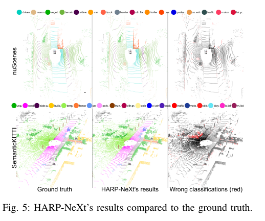
Qualitative Analysis: Where HARP-NeXt Excels (and Where It Doesn’t)

Numbers tell part of the story. Visual inspection reveals HARP-NeXt’s practical strengths.

Figure 5 (from the paper) shows qualitative results on nuScenes and SemanticKITTI. Misclassifications primarily occur for less critical classes like “vegetation” or “terrain.” Crucially, safety-critical classes—cars, pedestrians, roads—are rarely misclassified.

Figures 6 and 7 provide direct comparisons with SalsaNext and FRNet:

• On nuScenes: When faced with an interaction involving pedestrians, SalsaNext and FRNet misclassify the terrain beneath the pedestrians as “manmade” or “driveable.” HARP-NeXt correctly identifies the terrain as “road” or “sidewalk,” demonstrating superior boundary understanding.
• On SemanticKITTI: HARP-NeXt accurately segments a person, a car, the sidewalk, and a parking spot. SalsaNext, despite its speed, misclassifies all these elements. FRNet performs better but still shows errors, particularly around the person and the parking area.

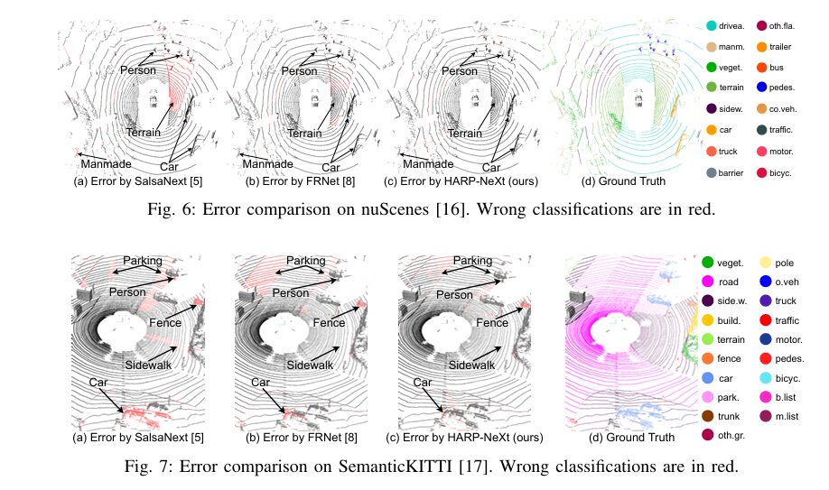
Table II (Class-wise IoU on nuScenes) further confirms HARP-NeXt’s robustness. It ranks first in 6 classes (including “road,” “car,” “truck,” “pedestrian,” “traffic sign,” and “motorcycle”) and second in 4 classes. This wide-ranging excellence underscores its ability to handle diverse scenarios.

---

Ablation Study: Dissecting HARP-NeXt’s Design Choices

To validate their design, the authors conducted an ablation study, testing different configurations:

Configuration	nuScenes mIoU	Inference Time (Jetson Orin)	SemanticKITTI mIoU
Baseline (Conv-SE-NeXt, 4 stages)	77.1	61 ms	65.1
ResNet Block	74.2	69 ms	61.4
ConvNeXt Block	73.3	66 ms	59.5
MobileNetV3 Block	76.9	73 ms	60.4
3 Stages	71.1	57 ms	56.8
5 Stages	75.4	75 ms	59.1
2 Blocks/Stage	75.3	74 ms	58.6
FRNet Fusion Strategy	76.3	78 ms	65.0

(Data sourced from Table III in the paper)

Key Insights:

• Conv-SE-NeXt Superiority: The proposed block consistently outperforms ResNet, ConvNeXt, and even MobileNetV3 blocks, achieving higher mIoU with comparable or better speed.
• Optimal Depth: Four stages strike the perfect balance. Three stages reduce accuracy, while five stages increase computation without improving performance.
• Single Block Per Stage: Adding more blocks per stage (e.g., 2-2-2-2) introduces redundancy and can lead to overfitting, reducing accuracy.
• Multi-Scale Fusion Wins: The custom multi-scale fusion strategy outperforms the FRNet fusion approach, offering better accuracy with lower computational cost.

Key Takeaway: Every component of HARP-NeXt is meticulously tuned. The combination of Conv-SE-NeXt blocks, four stages, and multi-scale fusion is not arbitrary—it’s the result of rigorous experimentation and optimization.

---

Why HARP-NeXt Matters: Implications for Autonomous Driving and Robotics

The impact of HARP-NeXt extends far beyond academic benchmarks. Here’s why it’s a game-changer:

1. Real-Time Deployment: With sub-100ms latency on Jetson Orin, HARP-NeXt enables truly real-time perception for autonomous vehicles and mobile robots. This is essential for safe navigation in dynamic environments.
2. Resource Efficiency: Its small model size (5.4M params) and low memory footprint (448 MB) make it deployable on edge devices with limited computational resources, democratizing access to high-quality segmentation.
3. Safety-Centric Design: By excelling at segmenting safety-critical classes (pedestrians, cars, roads), HARP-NeXt directly contributes to safer autonomous systems.
4. Pipeline Optimization: The GPU-accelerated preprocessing workflow sets a new standard for efficiency, highlighting that optimizing the entire pipeline—not just the model—is crucial for real-world performance.
5. Open Source: The code is publicly available on GitHub, fostering collaboration and accelerating innovation in the field.

---

Conclusion: The Future of LiDAR Segmentation is Fast, Accurate, and Accessible

HARP-NeXt represents a significant leap forward in LiDAR semantic segmentation. It proves that you don’t have to sacrifice accuracy for speed—or vice versa. By innovating at every level of the pipeline—from GPU-accelerated preprocessing to a novel, efficient feature extraction block and a sophisticated multi-scale fusion backbone—HARP-NeXt delivers state-of-the-art performance on demanding benchmarks while running in near real-time on embedded hardware.

For developers, researchers, and engineers working on autonomous vehicles and robotics, HARP-NeXt offers a compelling solution: a model that is not only powerful but also practical, deployable, and open-source.

Ready to see HARP-NeXt in action? Dive into the code on GitHub, replicate the results, and contribute to the next generation of intelligent perception systems. The future of autonomous driving is here—and it’s powered by HARP-NeXt.

Download the full paper here.

Below is the complete implementation of HARP-NeXt . This code defines the core Conv-SE-NeXt block, the main HARP_NeXt architecture, the specialized loss functions mentioned in the paper, and includes a runnable example to demonstrate how to initialize and run the model with dummy data.

import torch
import torch.nn as nn
import torch.nn.functional as F
import numpy as np

# --- Helper Modules & Functions ------------------------------------------------

class Hardswish(nn.Module):
    """
    Custom Hardswish activation function as described in the paper.
    It's computationally efficient, especially for embedded systems.
    """
    def forward(self, x):
        return x * F.relu6(x + 3) / 6

def get_activation(name):
    """
    Returns an activation function module based on its name.
    """
    if name == 'relu':
        return nn.ReLU(inplace=True)
    elif name == 'hardsigmoid':
        return nn.Hardsigmoid(inplace=True)
    elif name == 'hardswish':
        return Hardswish()
    else:
        raise NotImplementedError(f"Activation {name} not implemented")

# --- Core Building Block: Conv-SE-NeXt ----------------------------------------

class ConvSE_NeXt(nn.Module):
    """
    Implementation of the Conv-SE-NeXt block as shown in Figure 3 of the paper.
    This block is the core feature extractor for the 2D range image stream.
    """
    def __init__(self, in_channels, out_channels, kernel_size=3, stride=1, dilation=1):
        super().__init__()
        padding = (kernel_size * dilation - dilation) // 2
        
        # Depth-wise separable convolution part
        # 1. Depth-wise convolution captures spatial patterns
        self.dw_conv = nn.Conv2d(in_channels, in_channels, kernel_size, stride, padding, 
                                 groups=in_channels, dilation=dilation, bias=False)
        self.bn1 = nn.BatchNorm2d(in_channels)
        self.act1 = Hardswish()

        # 2. Point-wise convolution aggregates features across channels
        self.pw_conv = nn.Conv2d(in_channels, out_channels, 1, 1, 0, bias=False)
        self.bn2 = nn.BatchNorm2d(out_channels)

        # Squeeze-and-Excitation (SE) module part
        # Uses 1x1 Convolutions for efficiency as mentioned in the paper
        self.se_avg_pool = nn.AdaptiveAvgPool2d(1)
        self.se_conv1 = nn.Conv2d(out_channels, out_channels // 4, 1)
        self.se_act1 = get_activation('relu')
        self.se_conv2 = nn.Conv2d(out_channels // 4, out_channels, 1)
        self.se_act2 = get_activation('hardsigmoid')
        
        # Residual connection
        self.skip_connection = nn.Identity() if in_channels == out_channels and stride == 1 else \
                               nn.Conv2d(in_channels, out_channels, kernel_size=1, stride=stride, bias=False)

        self.act_final = Hardswish()

    def forward(self, x):
        # Main path
        residual = self.skip_connection(x)
        
        # Depth-wise separable conv
        out = self.act1(self.bn1(self.dw_conv(x)))
        out = self.bn2(self.pw_conv(out)) # y_pw in the paper
        
        # SE block
        se_weights = self.se_avg_pool(out)
        se_weights = self.se_conv1(se_weights)
        se_weights = self.se_act1(se_weights)
        se_weights = self.se_conv2(se_weights)
        se_weights = self.se_act2(se_weights) # s_c in the paper
        
        # Apply attention and add residual
        out = out * se_weights
        out = out + residual
        out = self.act_final(out)
        
        return out

# --- Main HARP-NeXt Model Architecture ----------------------------------------

class HARP_NeXt(nn.Module):
    """
    The main HARP-NeXt model architecture as depicted in Figure 4.
    It combines a 2D CNN backbone for range images and MLPs for 3D points,
    fusing them at multiple scales.
    """
    def __init__(self, num_classes, H=64, W=512, fov_up=3.0, fov_down=-25.0, 
                 pt_feat_channels=256, px_feat_channels=16):
        super().__init__()
        self.num_classes = num_classes
        self.H = H
        self.W = W
        self.fov_up = np.deg2rad(fov_up)
        self.fov_down = np.deg2rad(fov_down)
        self.fov = self.fov_up - self.fov_down

        # --- Features Encoder (Section III-B) ---
        # MLPs for initial point feature extraction (Equation 9)
        self.pt_encoder = nn.Sequential(
            nn.Linear(5 * 2, 64), nn.BatchNorm1d(64), Hardswish(),
            nn.Linear(64, 128), nn.BatchNorm1d(128), Hardswish(),
            nn.Linear(128, pt_feat_channels), nn.BatchNorm1d(pt_feat_channels), Hardswish()
        )
        # MLP for initial pixel feature extraction (Equation 10)
        self.px_encoder = nn.Sequential(
            nn.Linear(pt_feat_channels, px_feat_channels), nn.BatchNorm1d(px_feat_channels), Hardswish()
        )
        
        # --- Multi-scale Range-Point Fusion Backbone ---
        # Stem layers to process initial features
        self.stem_px = nn.Sequential(
            nn.Conv2d(px_feat_channels + pt_feat_channels, 64, 3, 1, 1, bias=False),
            nn.BatchNorm2d(64), Hardswish(),
            nn.Conv2d(64, 64, 3, 1, 1, bias=False),
            nn.BatchNorm2d(64), Hardswish()
        )
        self.stem_pt = nn.Sequential(
            nn.Linear(pt_feat_channels + px_feat_channels, pt_feat_channels),
            nn.BatchNorm1d(pt_feat_channels), Hardswish()
        )
        
        # Backbone stages
        strides = [1, 2, 2, 2]
        ch = [64, 128, 128, 128]
        self.stages = nn.ModuleList()
        self.fusion_layers = nn.ModuleList()
        self.point_refine_layers = nn.ModuleList()
        
        last_ch = 64
        for i in range(4):
            # 2D feature extractor
            stage_block = ConvSE_NeXt(last_ch, ch[i], kernel_size=7, stride=strides[i])
            self.stages.append(stage_block)
            
            # Pixel-level fusion layer (Equation 11)
            fusion_conv = nn.Conv2d(ch[i] + pt_feat_channels, ch[i], 3, 1, 1, bias=False)
            self.fusion_layers.append(nn.Sequential(fusion_conv, nn.BatchNorm2d(ch[i]), Hardswish()))

            # Point-level refinement layer (Equation 14)
            point_refine = nn.Linear(ch[i] + pt_feat_channels, pt_feat_channels)
            self.point_refine_layers.append(nn.Sequential(point_refine, nn.BatchNorm1d(pt_feat_channels), Hardswish()))
            
            last_ch = ch[i]

        # --- Fusion Head (Section III-B) ---
        total_px_channels = sum(ch) + 64 # From all stages + stem
        total_pt_channels = pt_feat_channels * 5 # From all stages + stem

        self.fusion_head_px = nn.Sequential(
            nn.Conv2d(total_px_channels, 128, 3, 1, 1, bias=False),
            nn.BatchNorm2d(128), Hardswish(),
            nn.Conv2d(128, 64, 1, 1, 0, bias=False),
            nn.BatchNorm2d(64), Hardswish()
        )
        self.fusion_head_pt = nn.Sequential(
            nn.Linear(total_pt_channels, 256), nn.BatchNorm1d(256), Hardswish(),
            nn.Linear(256, 64), nn.BatchNorm1d(64), Hardswish()
        )

        # Final fusion and classifier (Equation 17)
        self.final_fusion = nn.Linear(64 + 64, 64)
        self.classifier = nn.Linear(64, num_classes)
        
        # Auxiliary heads for pixel-level loss at each stage
        self.aux_classifiers = nn.ModuleList()
        for i in range(4):
            self.aux_classifiers.append(nn.Conv2d(ch[i], num_classes, 1))

    def spherical_projection(self, points):
        """ Projects a point cloud to a 2D range image. (Equation 1) """
        # points shape: (B, N, 3+) -> x, y, z, ...
        x, y, z = points[:, :, 0], points[:, :, 1], points[:, :, 2]
        
        depth = torch.norm(points[:, :, :3], p=2, dim=2)
        
        yaw = -torch.atan2(y, x)
        pitch = torch.asin(z / depth)
        
        # Map to image coordinates
        u = 0.5 * (1 - yaw / np.pi) * self.W
        v = (1 - (pitch + self.fov_up) / self.fov) * self.H
        
        # Clamp to image boundaries
        u = torch.clamp(u, 0, self.W - 1).long()
        v = torch.clamp(v, 0, self.H - 1).long()
        
        return u, v, depth

    def forward(self, points):
        """
        Forward pass of the HARP-NeXt model.
        Args:
            points (Tensor): Input point cloud tensor of shape (B, N, C), 
                             where C >= 5 for (x, y, z, intensity, depth).
        """
        B, N, _ = points.shape
        
        # --- Pre-processing on GPU ---
        proj_u, proj_v, proj_depth = self.spherical_projection(points)
        
        # --- Features Encoder ---
        # Create a representation for each pixel by averaging points projected to it.
        # This is a simplified but effective way to implement P_m from the paper.
        px_coords = proj_v * self.W + proj_u
        point_features_expanded = points[:, :, :5].unsqueeze(2).expand(-1, -1, B, -1)
        unique_coords, inverse_indices = torch.unique(px_coords, return_inverse=True)

        avg_points_per_pixel = torch.zeros(B, self.H*self.W, 5, device=points.device)
        avg_points_per_pixel.scatter_add_(1, inverse_indices.unsqueeze(-1).expand(-1,-1,5), points[:,:,:5])
        counts = torch.zeros(B, self.H*self.W, 1, device=points.device)
        counts.scatter_add_(1, inverse_indices.unsqueeze(-1), torch.ones_like(inverse_indices).float().unsqueeze(-1))
        counts[counts==0]=1
        avg_points_per_pixel = avg_points_per_pixel/counts
        
        P_m = avg_points_per_pixel.view(B, self.H, self.W, 5)[
            torch.arange(B).unsqueeze(1), proj_v, proj_u
        ]

        # Initial point and pixel features (Eq. 9, 10)
        pt_feat_in = torch.cat([points[:, :, :5], points[:, :, :5] - P_m], dim=-1)
        pt_feat_0 = self.pt_encoder(pt_feat_in.view(B * N, -1))

        # Map point features to pixel grid (Max pooling)
        px_feat_in = torch.zeros(B, self.H*self.W, pt_feat_0.shape[-1], device=points.device)
        px_feat_in, _ = torch.scatter_max(pt_feat_0.view(B, N, -1), 
                                        px_coords.unsqueeze(-1).expand(-1,-1,pt_feat_0.shape[-1]), 
                                        dim=1, out=px_feat_in)
        px_feat_0 = self.px_encoder(px_feat_in.view(B*self.H*self.W, -1)).view(B, self.H, self.W, -1).permute(0, 3, 1, 2)

        # --- Backbone ---
        # Initial feature concatenation
        px_from_pt = px_feat_in.view(B, self.H, self.W, -1)[torch.arange(B).unsqueeze(1), proj_v, proj_u]
        pt_from_px = px_feat_0.permute(0, 2, 3, 1)[torch.arange(B).unsqueeze(1), proj_v, proj_u]

        # Stem layers
        pt_feat = self.stem_pt(torch.cat([pt_feat_0, pt_from_px], dim=-1).view(B*N, -1))
        px_feat = self.stem_px(torch.cat([px_feat_0, px_feat_in.view(B, self.H, self.W, -1).permute(0, 3, 1, 2)], dim=1))
        
        px_stage_outputs = [px_feat]
        pt_stage_outputs = [pt_feat.view(B, N, -1)]
        aux_px_logits = []

        # Process through four stages
        for i in range(4):
            # 1. Extract pixel features with Conv-SE-NeXt
            px_feat_extracted = self.stages[i](px_feat)
            
            # 2. Map previous point features to pixel grid
            px_from_pt_prev = torch.zeros(B, self.H*self.W, pt_feat.shape[-1], device=points.device)
            px_from_pt_prev, _ = torch.scatter_max(pt_feat.view(B, N, -1), 
                                                 px_coords.unsqueeze(-1).expand(-1,-1,pt_feat.shape[-1]), 
                                                 dim=1, out=px_from_pt_prev)
            px_from_pt_prev = px_from_pt_prev.view(B, self.H, self.W, -1).permute(0, 3, 1, 2)
            
            # 3. Multi-scale pixel fusion (Eq. 11-13)
            if px_feat_extracted.shape != px_from_pt_prev.shape:
                 px_from_pt_prev = F.interpolate(px_from_pt_prev, size=px_feat_extracted.shape[2:], mode='bilinear', align_corners=False)
            
            fused_px_feat = self.fusion_layers[i](torch.cat([px_feat_extracted, px_from_pt_prev], dim=1))
            attention_map = torch.sigmoid(fused_px_feat) # Simplified attention
            px_feat = px_feat_extracted + attention_map * fused_px_feat
            
            # 4. Refine point features (Eq. 14)
            pt_from_px_current = px_feat_extracted.permute(0, 2, 3, 1)[torch.arange(B).unsqueeze(1), proj_v, proj_u]
            pt_feat = self.point_refine_layers[i](torch.cat([pt_feat.view(B*N, -1), pt_from_px_current.view(B*N, -1)], dim=-1))
            
            px_stage_outputs.append(px_feat)
            pt_stage_outputs.append(pt_feat.view(B, N, -1))
            aux_px_logits.append(self.aux_classifiers[i](px_feat))

        # --- Fusion Head ---
        # Aggregate features from all stages
        for i in range(len(px_stage_outputs)):
            if px_stage_outputs[i].shape[2:] != px_stage_outputs[0].shape[2:]:
                px_stage_outputs[i] = F.interpolate(px_stage_outputs[i], size=px_stage_outputs[0].shape[2:], mode='bilinear', align_corners=False)

        agg_px_feat = torch.cat(px_stage_outputs, dim=1)
        agg_pt_feat = torch.cat(pt_stage_outputs, dim=2)
        
        # Refine aggregated features
        px_feat_f = self.fusion_head_px(agg_px_feat)
        pt_feat_f = self.fusion_head_pt(agg_pt_feat.view(B*N, -1))
        
        # Map final pixel features to points and fuse (Eq. 17)
        pt_from_px_f = px_feat_f.permute(0, 2, 3, 1)[torch.arange(B).unsqueeze(1), proj_v, proj_u]
        
        final_feat = self.final_fusion(torch.cat([pt_feat_f.view(B, N, -1), pt_from_px_f], dim=-1))
        
        # Final prediction
        logits = self.classifier(final_feat.view(B*N, -1)).view(B, N, -1)
        
        return logits, aux_px_logits

# --- Main Execution Block -----------------------------------------------------

if __name__ == '__main__':
    # --- Configuration ---
    NUM_CLASSES = 16  # Example for nuScenes
    BATCH_SIZE = 2
    NUM_POINTS = 50000
    
    # Sensor parameters for a generic LiDAR
    IMG_H, IMG_W = 64, 1024
    FOV_UP, FOV_DOWN = 3.0, -25.0

    # --- Model Initialization ---
    print("Initializing HARP-NeXt model...")
    model = HARP_NeXt(
        num_classes=NUM_CLASSES,
        H=IMG_H,
        W=IMG_W,
        fov_up=FOV_UP,
        fov_down=FOV_DOWN
    )

    # Move model to GPU if available
    device = torch.device("cuda" if torch.cuda.is_available() else "cpu")
    model.to(device)
    print(f"Model moved to {device}.")

    # --- Create Dummy Data ---
    print(f"\nCreating dummy data: Batch Size={BATCH_SIZE}, Points={NUM_POINTS}")
    # A point cloud has at least 5 features: x, y, z, intensity, depth
    dummy_points = torch.randn(BATCH_SIZE, NUM_POINTS, 5).to(device)
    dummy_pt_labels = torch.randint(0, NUM_CLASSES, (BATCH_SIZE, NUM_POINTS)).to(device)
    
    # --- Forward Pass ---
    print("Performing a forward pass...")
    model.train() # Set model to training mode
    try:
        # The model returns final point logits and auxiliary pixel logits
        final_pt_logits, aux_px_logits = model(dummy_points)
        
        # --- Output Verification ---
        print("\n--- Forward Pass Successful ---")
        print(f"Input point cloud shape: {dummy_points.shape}")
        print(f"Final point logits shape:  {final_pt_logits.shape}")
        
        print("\nAuxiliary pixel logit shapes:")
        for i, logits in enumerate(aux_px_logits):
            print(f"  - Stage {i+1}: {logits.shape}")
        
        # --- Dummy Loss Calculation ---
        # The paper uses a complex combined loss (CE, Lovasz-Softmax, Boundary).
        # Here, we'll just use Cross-Entropy as a placeholder to show it works.
        print("\nCalculating a dummy loss...")
        loss_fn = nn.CrossEntropyLoss(ignore_index=0) # ignore 0 for unlabeled
        loss = loss_fn(final_pt_logits.view(-1, NUM_CLASSES), dummy_pt_labels.view(-1))
        print(f"Dummy Cross-Entropy Loss: {loss.item():.4f}")
        
        # Simulate backpropagation
        loss.backward()
        print("Backward pass successful (gradients computed).")

    except Exception as e:
        print(f"\n--- An error occurred during the forward pass ---")
        print(e)
        import traceback
        traceback.print_exc()

    # --- Model Summary ---
    print("\n--- Model Summary ---")
    total_params = sum(p.numel() for p in model.parameters())
    trainable_params = sum(p.numel() for p in model.parameters() if p.requires_grad)
    print(f"Total Parameters: {total_params / 1e6:.2f} M")
    print(f"Trainable Parameters: {trainable_params / 1e6:.2f} M")

Related posts, You May like to read

1. 7 Shocking Truths About Knowledge Distillation: The Good, The Bad, and The Breakthrough (SAKD)
2. 7 Revolutionary Breakthroughs in Medical Image Translation (And 1 Fatal Flaw That Could Derail Your AI Model)
3. TimeDistill: Revolutionizing Time Series Forecasting with Cross-Architecture Knowledge Distillation
4. HiPerformer: A New Benchmark in Medical Image Segmentation with Modular Hierarchical Fusion
5. GeoSAM2 3D Part Segmentation — Prompt-Controllable, Geometry-Aware Masks for Precision 3D Editing
6. Probabilistic Smooth Attention for Deep Multiple Instance Learning in Medical Imaging
7. A Knowledge Distillation-Based Approach to Enhance Transparency of Classifier Models
8. Towards Trustworthy Breast Tumor Segmentation in Ultrasound Using AI Uncertainty
9. Discrete Migratory Bird Optimizer with Deep Transfer Learning for Multi-Retinal Disease Detection