When a deep learning model trained to detect tuberculosis in chest X-rays encounters an image with slightly lower contrast or minor sensor noise, it often fails catastrophically—sometimes with confidence scores above 90%. This fragility isn’t just a technical inconvenience; in clinical settings, it represents a critical patient safety issue. The gap between pristine research datasets and chaotic real-world medical imaging has long undermined the deployment of artificial intelligence in radiology and dermatology.
Enter LaDiNE (Latent-guided Diffusion Nested-Ensembles), a groundbreaking framework recently introduced in IEEE Transactions on Medical Imaging that fundamentally reimagines how medical AI systems handle uncertainty and distribution shifts. By synergistically combining the hierarchical feature extraction of Vision Transformers (ViTs) with the probabilistic power of diffusion models, LaDiNE achieves unprecedented robustness against unseen covariate shifts while maintaining calibrated, trustworthy predictions.
The Critical Challenge: When Medical AI Meets Reality
Deep neural networks (DNNs) have achieved remarkable accuracy in controlled experimental settings, often matching or exceeding human performance in detecting diabetic retinopathy, skin cancer, and lung abnormalities. However, these models suffer from a fundamental brittleness: they assume that test data comes from the exact same distribution as training data. In practice, medical imaging equipment varies between hospitals, exposure settings fluctuate, and patient positioning introduces unpredictable variations.
Covariate shift—where the input distribution changes while the underlying pathology-label relationship remains constant—poses the single greatest threat to clinical AI deployment. Traditional data augmentation struggles to prepare models for these infinite real-world variations, especially when working with the small datasets common in rare disease research. When faced with Gaussian noise, resolution degradation, contrast adjustments, or adversarial perturbations, standard convolutional neural networks (CNNs) and even standard Vision Transformers often exhibit:
- Catastrophic accuracy drops (sometimes from 99% to 50% or lower)
- Poorly calibrated confidence (being wrong with high certainty)
- Vulnerability to adversarial attacks that could be exploited for insurance fraud or malicious purposes
LaDiNE: Architecture of a Robust Medical AI System
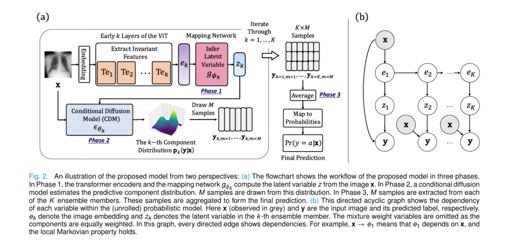
LaDiNE represents a paradigm shift from single-point deterministic predictions to probabilistic ensemble modeling through a novel parametric mixture approach. Unlike traditional deep ensembles that simply average the outputs of multiple independent networks, LaDiNE constructs a sophisticated hierarchical Bayesian network where each mixture component captures different levels of feature abstraction.
The Core Innovation: Diffusion Meets Transformers
At its heart, LaDiNE consists of three integrated components working in concert:
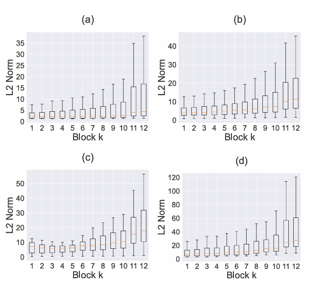
- Hierarchical Transformer Encoders: Unlike standard approaches that only use the final layer of a Vision Transformer, LaDiNE extracts features from early transformer encoder (TE) blocks. Research demonstrates that shallow layers capture invariant, low-level features (edges, textures) that remain stable under noise, while deeper layers encode fragile, high-level semantic information.
- Latent Mapping Networks: For each of the K ensemble members, a dedicated mapping network gk transforms the extracted features ek into latent variables zk that serve as robust conditioning signals.
- Conditional Diffusion Models (CDMs): Rather than assuming Gaussian predictive distributions (a common but restrictive simplification), LaDiNE employs diffusion models as flexible density estimators. These models learn the complex, heteroscedastic distributions of medical data through a denoising process conditioned on both the invariant latent features and the original image.
This architecture creates a functional-form-free predictive distribution, allowing the model to express complex uncertainty patterns that rigid parametric models cannot capture.
The Mathematical Foundation: Probabilistic Predictive Modeling
LaDiNE treats classification as a conditional density estimation problem. The predictive distribution is formulated as a mixture model with K components:
\[ p(\mathbf{y}|\mathbf{x}, \Theta) = \sum_{k=1}^{K} \pi_k \underbrace{\int \cdots \int p(\mathbf{y}, \mathbf{z}k, \mathbf{e}{1:k}|\mathbf{x}) , d\mathbf{z}k d\mathbf{e}{1:k}}_{\mathbf{p}_k(\mathbf{y}|\mathbf{x})} \]Each component distribution pk(y|x) factorizes through the latent hierarchy:
\[ \mathbf{p}k(\mathbf{y}|\mathbf{x}) = \int \cdots \int p{\theta_k}(\mathbf{y}|\mathbf{z}_k, \mathbf{x}) , p(\mathbf{z}_k|\mathbf{e}k) \prod{i=2}^{k} p(\mathbf{e}i|\mathbf{e}{i-1}) , p(\mathbf{e}_1|\mathbf{x}) , d\mathbf{z}k d\mathbf{e}{1:k} \]The Diffusion Process
The conditional diffusion model defines a forward Markov chain that gradually adds noise to the one-hot encoded label y0 over T timesteps:
\[ q(\mathbf{y}t|\mathbf{y}{t-1}, \mathbf{z}, \mathbf{x}) = \mathcal{N}\left(\mathbf{y}t; \sqrt{\alpha_t}\mathbf{y}{t-1} + (1-\sqrt{\alpha_t})(\mathbf{z} + \text{Enc}(\mathbf{x})), \beta_t \mathbf{I}\right) \]During inference, the model learns to reverse this process. The noise predictor ϵθ is trained via a simplified variational bound:
\[ \mathcal{L}{\text{CDM}}(\theta) = \mathbb{E}{\langle\mathbf{x}, \mathbf{y}_0\rangle, \epsilon, t} \left[ |\epsilon – \epsilon\theta(\mathbf{y}_t, \mathbf{z}, \mathbf{x}, t)|_2^2 \right] \]Where:
\[ \mathbf{y}_t = \sqrt{\bar{\alpha}_t}\mathbf{y}_0 + (1-\sqrt{\bar{\alpha}_t})(\mathbf{z} + \text{Enc}(\mathbf{x})) + \sqrt{1-\bar{\alpha}_t}\epsilon), with (\bar{\alpha}t = \prod{i=1}^t \alpha_i) \]This formulation allows LaDiNE to draw Monte Carlo samples from the predictive distribution, capturing epistemic uncertainty through the variance of these samples.
The Three-Phase Training Protocol
LaDiNE employs a sophisticated staged training strategy to prevent gradient conflicts between the components:
Phase 1: Vision Transformer Pre-training
The ViT backbone is trained end-to-end using standard cross-entropy loss on clean training images. This establishes a strong baseline feature extractor before freezing these parameters for subsequent phases.
Phase 2: Latent Variable Optimization
With the ViT frozen, each mapping network gk is trained to maximize the likelihood of the ground truth labels given the intermediate features ek. This ensures that zk contains both discriminative information and robustness to input perturbations.
Phase 3: Diffusion Model Training
Finally, with both the ViT and mapping networks frozen, the conditional diffusion models learn to denoise label vectors conditioned on the fixed latent representations. This separation prevents the diffusion process from “cheating” by adjusting the feature extractor, forcing it to genuinely model the conditional distribution p ( y|z, x).
Performance Under Pressure: Experimental Validation
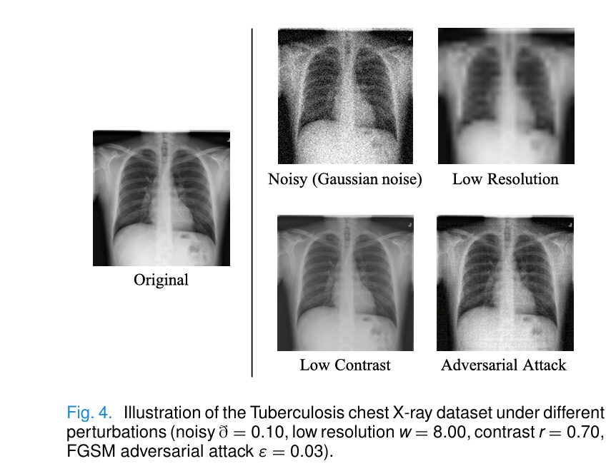
LaDiNE was rigorously evaluated on two challenging benchmarks: the Tuberculosis Chest X-ray Dataset (7,000 images) and the ISIC Skin Cancer Dataset (10,565 images). Unlike standard benchmarks that test only on clean data, the evaluation protocol subjected models to severe, previously unseen covariate shifts:Table
| Perturbation Type | LaDiNE Accuracy | Best Baseline | Performance Gap |
|---|---|---|---|
| Gaussian Noise (θ=1.00) | 73.16% | 50.00% (ResNet-50) | +23.16% |
| Low Resolution (factor 8) | 98.90% | 94.20% (ViT-B) | +4.70% |
| Low Contrast (ratio 0.70) | 93.14% | 91.50% (ResNet-50) | +1.64% |
| FGSM Attack (ϵ=0.03) | 94.86% | 85.90% (SEViT) | +8.96% |
Adversarial Robustness
Perhaps most impressively, LaDiNE demonstrates remarkable resilience to gradient-based adversarial attacks. When subjected to Projected Gradient Descent (PGD) and Auto-PGD attacks—sophisticated methods specifically designed to break neural networks—LaDiNE maintained accuracies above 96% on chest X-rays and 61% on skin cancer images. Competitors like ResNet-50 and EfficientNetV2-L collapsed to 0% accuracy under the same conditions.
This robustness stems from the diffusion model’s generative nature: by modeling the full predictive distribution rather than decision boundaries, adversarial perturbations must fundamentally alter the semantic content of the image to change the classification, moving beyond the “brittle features” vulnerable to gradient attacks.
Calibration and Clinical Trust: Beyond Raw Accuracy
In high-stakes medical diagnostics, calibration matters as much as accuracy. A model that claims 99% confidence should be correct 99% of the time. The Expected Calibration Error (ECE) measures this alignment:
\[ \text{ECE}b = \sum{i=1}^{b} \frac{|B_i|}{n} \left| \text{acc}(B_i) – \text{conf}(B_i) \right| \]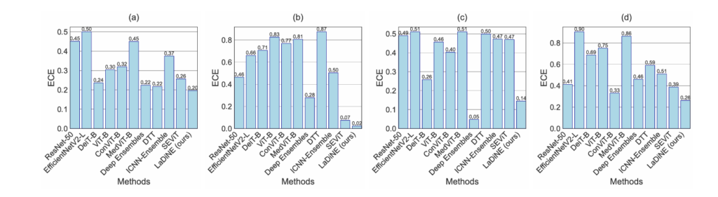
LaDiNE achieves the lowest ECE across all tested perturbations, ensuring that when the model expresses high confidence, clinicians can trust the prediction. Conversely, the framework provides meaningful instance-level uncertainty quantification through two metrics:
- Class-wise Prediction Interval Width (CPIW): Measures the spread of samples drawn from the diffusion model. Wider intervals indicate higher uncertainty.
- Class-wise Normalized Prediction Variance (CNPV): Quantifies consistency across ensemble members.
In experiments with severely noisy images (\(\sigma=1.00\)), LaDiNE correctly assigned higher uncertainty (CPIW = 0.86) to incorrect predictions while maintaining lower variance (CPIW = 0.43) for correct tuberculosis detections, enabling effective triage for human review.
Limitations and Future Directions
Despite its breakthrough performance, LaDiNE faces practical deployment challenges. The iterative denoising process, while operating on the low-dimensional label space \(\mathbb{R}^A\) rather than pixel space, increases inference time to approximately 98ms per image on an NVIDIA A100 GPU, compared to 0.54ms for standard ViT-B.
Future research directions include:
- Accelerated Sampling: Integrating Denoising Diffusion Implicit Models (DDIM) or Consistency Models to reduce the number of required diffusion steps from 1000 to 50 or fewer.
- Parallelization: Distributing the K ensemble members across multiple GPUs to reduce latency.
- Bayesian Extensions: Incorporating Bayesian Neural Networks to handle weight uncertainty alongside data uncertainty, potentially stabilizing the slight initialization sensitivity observed in the current implementation.
Conclusion: A New Standard for Medical AI
LaDiNE represents more than an incremental improvement in medical image classification—it establishes a new paradigm where robustness, calibration, and uncertainty quantification are architectural priorities rather than afterthoughts. By leveraging the complementary strengths of Vision Transformers (invariant feature extraction) and diffusion models (flexible density estimation), the framework provides a blueprint for trustworthy AI in clinical environments where “good enough” accuracy is never good enough.
As medical AI transitions from research curiosity to clinical necessity, frameworks like LaDiNE that explicitly account for the messy, noisy reality of healthcare data will become the gold standard. For researchers and practitioners looking to bridge the gap between laboratory performance and bedside reliability, adopting diffusion-based ensemble methods offers a clear path forward.
What challenges have you encountered with AI robustness in medical imaging? Share your experiences in the comments below, or subscribe to our newsletter for deep dives into the latest advances in clinical machine learning.
import torch
import torch.nn as nn
import torch.nn.functional as F
import torch.optim as optim
from torch.utils.data import DataLoader
import math
import numpy as np
from typing import Optional, Tuple, List
# =============================================================================
# Component 1: Vision Transformer (ViT) Backbone
# =============================================================================
class PatchEmbedding(nn.Module):
def __init__(self, img_size=224, patch_size=16, in_channels=3, embed_dim=768):
super().__init__()
self.img_size = img_size
self.patch_size = patch_size
self.n_patches = (img_size // patch_size) ** 2
self.proj = nn.Conv2d(in_channels, embed_dim, kernel_size=patch_size, stride=patch_size)
self.cls_token = nn.Parameter(torch.randn(1, 1, embed_dim))
self.pos_embed = nn.Parameter(torch.randn(1, self.n_patches + 1, embed_dim))
self.dropout = nn.Dropout(0.1)
def forward(self, x):
B, C, H, W = x.shape
x = self.proj(x).flatten(2).transpose(1, 2) # (B, n_patches, embed_dim)
cls_tokens = self.cls_token.expand(B, -1, -1) # (B, 1, embed_dim)
x = torch.cat([cls_tokens, x], dim=1) # (B, n_patches+1, embed_dim)
x = x + self.pos_embed
x = self.dropout(x)
return x
class TransformerEncoder(nn.Module):
def __init__(self, embed_dim=768, num_heads=12, mlp_ratio=4.0, dropout=0.1):
super().__init__()
self.norm1 = nn.LayerNorm(embed_dim)
self.attn = nn.MultiheadAttention(embed_dim, num_heads, dropout=dropout, batch_first=True)
self.norm2 = nn.LayerNorm(embed_dim)
self.mlp = nn.Sequential(
nn.Linear(embed_dim, int(embed_dim * mlp_ratio)),
nn.GELU(),
nn.Dropout(dropout),
nn.Linear(int(embed_dim * mlp_ratio), embed_dim),
nn.Dropout(dropout)
)
def forward(self, x):
# Self-attention with residual
x2 = self.norm1(x)
attn_out, _ = self.attn(x2, x2, x2)
x = x + attn_out
# MLP with residual
x = x + self.mlp(self.norm2(x))
return x
class ViTBackbone(nn.Module):
def __init__(self, img_size=224, patch_size=16, in_channels=3, embed_dim=768,
depth=12, num_heads=12, mlp_ratio=4.0, num_classes=2, dropout=0.1):
super().__init__()
self.patch_embed = PatchEmbedding(img_size, patch_size, in_channels, embed_dim)
self.encoders = nn.ModuleList([
TransformerEncoder(embed_dim, num_heads, mlp_ratio, dropout)
for _ in range(depth)
])
self.norm = nn.LayerNorm(embed_dim)
self.head = nn.Linear(embed_dim, num_classes)
self.depth = depth
def forward(self, x, return_intermediate=None):
"""
Args:
x: Input images (B, C, H, W)
return_intermediate: If True, return embeddings from all blocks
Returns:
logits: Classification logits
intermediate_features: List of embeddings [e_1, e_2, ..., e_K] if requested
"""
x = self.patch_embed(x)
B = x.shape[0]
intermediate_features = []
for i, encoder in enumerate(self.encoders):
x = encoder(x)
# Extract features after each block (excluding cls token for latent features)
if return_intermediate:
# e_i is the embedding excluding cls token: (B, n_patches, embed_dim)
intermediate_features.append(x[:, 1:, :])
x = self.norm(x)
cls_token = x[:, 0]
logits = self.head(cls_token)
if return_intermediate:
return logits, intermediate_features
return logits
# =============================================================================
# Component 2: Mapping Network (g_phi)
# =============================================================================
class MappingNetwork(nn.Module):
"""
Maps embedding e_k to latent variable z_k
MLP with 3 hidden layers as specified in paper
"""
def __init__(self, embed_dim=768, latent_dim=128, num_classes=2, hidden_dim=512):
super().__init__()
self.mlp = nn.Sequential(
nn.Linear(embed_dim, hidden_dim),
nn.ReLU(),
nn.Dropout(0.1),
nn.Linear(hidden_dim, hidden_dim),
nn.ReLU(),
nn.Dropout(0.1),
nn.Linear(hidden_dim, hidden_dim),
nn.ReLU(),
nn.Dropout(0.1),
nn.Linear(hidden_dim, latent_dim)
)
# Projection to class logits for training Step 2
self.logit_proj = nn.Linear(latent_dim, num_classes)
def forward(self, e_k):
"""
Args:
e_k: (B, N, embed_dim) where N is number of patches
Returns:
z_k: (B, latent_dim) - pooled latent variable
logits: (B, num_classes) - for training Step 2
"""
# Global average pooling over patches
e_k_pooled = e_k.mean(dim=1) # (B, embed_dim)
z_k = self.mlp(e_k_pooled) # (B, latent_dim)
logits = self.logit_proj(z_k) # (B, num_classes)
return z_k, logits
# =============================================================================
# Component 3: Conditional Diffusion Model (CDM)
# =============================================================================
class TimeEmbedding(nn.Module):
def __init__(self, dim):
super().__init__()
self.dim = dim
def forward(self, time):
device = time.device
half_dim = self.dim // 2
embeddings = math.log(10000) / (half_dim - 1)
embeddings = torch.exp(torch.arange(half_dim, device=device) * -embeddings)
embeddings = time[:, None] * embeddings[None, :]
embeddings = torch.cat([embeddings.sin(), embeddings.cos()], dim=-1)
return embeddings
class ImageEncoder(nn.Module):
"""
Encodes image x into same dimension as z for CDM conditioning
"""
def __init__(self, img_size=224, in_channels=3, embed_dim=128):
super().__init__()
# Simple CNN encoder or could use ViT features
self.encoder = nn.Sequential(
nn.Conv2d(in_channels, 64, 7, stride=2, padding=3),
nn.ReLU(),
nn.MaxPool2d(2),
nn.Conv2d(64, 128, 3, stride=2, padding=1),
nn.ReLU(),
nn.AdaptiveAvgPool2d(1),
nn.Flatten(),
nn.Linear(128, embed_dim)
)
def forward(self, x):
return self.encoder(x)
class ConditionalDiffusionModel(nn.Module):
"""
Noise predictor epsilon_theta(y_t, z, x, t)
MLP with 3 hidden layers using element-wise product for conditioning
"""
def __init__(self, num_classes=2, latent_dim=128, time_dim=128, hidden_dim=512):
super().__init__()
self.time_embed = TimeEmbedding(time_dim)
# Project time embedding
self.time_proj = nn.Sequential(
nn.Linear(time_dim, hidden_dim),
nn.SiLU(),
nn.Linear(hidden_dim, hidden_dim)
)
# Image encoder to condition on x
self.image_encoder = ImageEncoder(embed_dim=latent_dim)
# Main network: takes concatenated [y_t, z, Enc(x)] with time conditioning
input_dim = num_classes + latent_dim + latent_dim # y_t + z + Enc(x)
self.net = nn.Sequential(
nn.Linear(input_dim + hidden_dim, hidden_dim), # +hidden_dim for time
nn.ReLU(),
nn.Dropout(0.1),
nn.Linear(hidden_dim, hidden_dim),
nn.ReLU(),
nn.Dropout(0.1),
nn.Linear(hidden_dim, hidden_dim),
nn.ReLU(),
nn.Dropout(0.1),
nn.Linear(hidden_dim, num_classes) # Predict noise for each class dimension
)
def forward(self, y_t, z, x, t):
"""
Args:
y_t: (B, num_classes) - noisy label at timestep t
z: (B, latent_dim) - latent from mapping network
x: (B, C, H, W) - input image
t: (B,) - timestep
Returns:
noise: (B, num_classes) - predicted noise
"""
t_emb = self.time_proj(self.time_embed(t))
x_enc = self.image_encoder(x)
# Concatenate features
features = torch.cat([y_t, z, x_enc], dim=1) # (B, num_classes + 2*latent_dim)
# Element-wise product conditioning (as mentioned in paper)
# Here implemented as concatenation + interaction through network
h = torch.cat([features, t_emb], dim=1)
noise = self.net(h)
return noise
# =============================================================================
# LaDiNE: Complete Model
# =============================================================================
class LaDiNE(nn.Module):
def __init__(self, img_size=224, patch_size=16, in_channels=3, embed_dim=768,
vit_depth=12, num_heads=12, num_classes=2, K=5, latent_dim=128,
diffusion_steps=1000, beta_start=1e-4, beta_end=0.02):
super().__init__()
self.K = K # Number of ensemble members (mixture components)
self.num_classes = num_classes
self.latent_dim = latent_dim
self.T = diffusion_steps
# Vision Transformer Backbone
self.vit = ViTBackbone(img_size, patch_size, in_channels, embed_dim,
vit_depth, num_heads, num_classes=num_classes)
# Mapping networks for each ensemble member (each uses different TE block output)
self.mapping_networks = nn.ModuleList([
MappingNetwork(embed_dim, latent_dim, num_classes)
for _ in range(K)
])
# Conditional Diffusion Models for each ensemble member
self.cdms = nn.ModuleList([
ConditionalDiffusionModel(num_classes, latent_dim)
for _ in range(K)
])
# Diffusion schedule (linear as per paper)
betas = torch.linspace(beta_start, beta_end, diffusion_steps)
self.register_buffer('betas', betas)
self.register_buffer('alphas', 1.0 - betas)
self.register_buffer('alphas_cumprod', torch.cumprod(1.0 - betas, dim=0))
self.register_buffer('sqrt_alphas_cumprod', torch.sqrt(self.alphas_cumprod))
self.register_buffer('sqrt_one_minus_alphas_cumprod', torch.sqrt(1.0 - self.alphas_cumprod))
def extract_features(self, x):
"""Extract intermediate features e_1 to e_K from ViT"""
_, features = self.vit(x, return_intermediate=True)
# Return first K features (paper uses early blocks for invariance)
return features[:self.K]
def get_latents(self, x):
"""Get latent variables z_k for all ensemble members"""
features = self.extract_features(x) # List of K features
latents = []
logits = []
for k in range(self.K):
z_k, logit_k = self.mapping_networks[k](features[k])
latents.append(z_k)
logits.append(logit_k)
return latents, logits, features
def q_sample(self, y_0, t, z, x_enc, noise=None):
"""
Forward diffusion process: q(y_t | y_0, z, x)
Implements equation from paper:
q(y_t | y_{t-1}) = N(sqrt(alpha_t)*y_{t-1} + (1-sqrt(alpha_t))*(z+x_enc), beta_t*I)
Reparameterized for direct sampling from y_0.
"""
if noise is None:
noise = torch.randn_like(y_0)
sqrt_alpha_t = torch.sqrt(self.alphas[t]).view(-1, 1)
one_minus_sqrt_alpha_t = 1 - sqrt_alpha_t
# Mean: sqrt(alpha_t)*y_0 + (1-sqrt(alpha_t))*(z + x_enc)
# Note: paper uses this specific parameterization for the shift toward conditioning
mean = sqrt_alpha_t * y_0 + one_minus_sqrt_alpha_t * (z + x_enc)
std = torch.sqrt(self.betas[t]).view(-1, 1)
return mean + std * noise
def forward_diffusion(self, y_0, t, z, x):
"""Sample y_t given y_0 using the cumulative product formula (reparameterization)"""
if noise is None:
noise = torch.randn_like(y_0)
sqrt_alphas_cumprod_t = self.sqrt_alphas_cumprod[t].view(-1, 1)
sqrt_one_minus_alphas_cumprod_t = self.sqrt_one_minus_alphas_cumprod[t].view(-1, 1)
# y_t = sqrt(bar_alpha_t)*y_0 + (1-sqrt(bar_alpha_t))*(z+x_enc) + sqrt(1-bar_alpha_t)*noise
# Adapted for cumulative form
x_enc = self.cdms[0].image_encoder(x) # Assume all CDMs share same encoder or use first
# In practice, each CDM has its own or shared Enc
mean = sqrt_alphas_cumprod_t * y_0 + (1 - sqrt_alphas_cumprod_t) * (z + x_enc)
return mean + sqrt_one_minus_alphas_cumprod_t * noise
def predict_noise(self, y_t, z, x, t, k):
"""Predict noise using k-th CDM"""
return self.cdms[k](y_t, z, x, t)
def p_sample(self, y_t, t, z, x, k):
"""
Reverse diffusion step: sample y_{t-1} from y_t
Implements Algorithm 1 from the paper
"""
B = y_t.shape[0]
device = y_t.device
alpha_t = self.alphas[t].view(-1, 1)
alpha_cumprod_t = self.alphas_cumprod[t].view(-1, 1)
alpha_cumprod_prev = self.alphas_cumprod[t - 1].view(-1, 1) if (t > 0).all() else torch.ones_like(alpha_cumprod_t)
beta_t = self.betas[t].view(-1, 1)
# Predict noise
eps_theta = self.predict_noise(y_t, z, x, t, k)
# Get Enc(x) for this CDM
x_enc = self.cdms[k].image_encoder(x)
# Compute estimated y_0 (Algorithm 1, line 3)
# tilde_y_0 = (1/sqrt(bar_alpha_t)) * (y_t - (1-sqrt(bar_alpha_t))*(z+x_enc) - sqrt(1-bar_alpha_t)*eps)
sqrt_alpha_cumprod_t = torch.sqrt(alpha_cumprod_t)
sqrt_one_minus_alpha_cumprod_t = torch.sqrt(1 - alpha_cumprod_t)
tilde_y_0 = (y_t - (1 - sqrt_alpha_cumprod_t) * (z + x_enc) -
sqrt_one_minus_alpha_cumprod_t * eps_theta) / sqrt_alpha_cumprod_t
if (t == 0).all():
return tilde_y_0
# Compute mu_q for y_{t-1} (Algorithm 1, line 6)
# Coefficients
coef1 = torch.sqrt(alpha_t) * (1 - alpha_cumprod_prev) / (1 - alpha_cumprod_t)
coef2 = beta_t * torch.sqrt(alpha_cumprod_prev) / (1 - alpha_cumprod_t)
coef3 = (torch.sqrt(alpha_t) * (1 - alpha_cumprod_prev) + beta_t * torch.sqrt(alpha_cumprod_prev)) / (1 - alpha_cumprod_t) - 1
mu = coef1 * y_t + coef2 * tilde_y_0 - coef3 * (z + x_enc)
# Variance
sigma_sq = beta_t * (1 - alpha_cumprod_prev) / (1 - alpha_cumprod_t)
sigma = torch.sqrt(sigma_sq)
noise = torch.randn_like(y_t)
return mu + sigma * noise
@torch.no_grad()
def sample_from_cdm(self, x, z, k, num_samples=20):
"""
Sample from p_theta_k(y | z_k, x) using Algorithm 1
Returns M samples for the k-th component
"""
B = x.shape[0]
device = x.device
samples = []
for m in range(num_samples):
# Line 1: Draw y_T ~ N(z, I)
y_t = z + torch.randn(B, self.num_classes).to(device)
# Lines 2-8: Reverse diffusion
for t in reversed(range(self.T)):
t_batch = torch.full((B,), t, device=device, dtype=torch.long)
y_t = self.p_sample(y_t, t_batch, z, x, k)
samples.append(y_t)
return torch.stack(samples, dim=1) # (B, M, num_classes)
def map_to_probability(self, y_avg, iota=0.1737):
"""
Map averaged prediction to probability simplex using Brier score-based mapping (Eq 18)
Args:
y_avg: (B, num_classes) - averaged predictions from MC sampling
iota: temperature parameter (tuned on validation set)
Returns:
probs: (B, num_classes)
"""
# Pr(y=a|x) = exp(-iota^{-1} * (y^a - 1)^2) / sum_i exp(-iota^{-1} * (y^i - 1)^2)
logits = -((y_avg - 1.0) ** 2) / iota
probs = F.softmax(logits, dim=1)
return probs
def forward(self, x, num_samples=20, iota=0.1737, return_uncertainty=False):
"""
Inference: Phase 1 -> Phase 2 -> Phase 3 (Algorithm aggregation)
Args:
x: Input images (B, C, H, W)
num_samples: M samples per component
iota: Calibration parameter
Returns:
probs: (B, num_classes) - final predicted probabilities
uncertainty: dict with CPIW and CNPV if requested
"""
B = x.shape[0]
device = x.device
# Phase 1: Compute latents z_k for all components
latents, _, _ = self.get_latents(x)
all_samples = []
# Phase 2: Draw M samples from each of K components
for k in range(self.K):
z_k = latents[k]
samples_k = self.sample_from_cdm(x, z_k, k, num_samples) # (B, M, num_classes)
all_samples.append(samples_k)
# Stack all samples: (B, K, M, num_classes)
all_samples = torch.stack(all_samples, dim=1)
# Phase 3: Aggregate
# Average all samples (Eq 16: (MK)^{-1} sum_k sum_m y_{k,m})
y_avg = all_samples.mean(dim=[1, 2]) # (B, num_classes)
# Map to probability simplex
probs = self.map_to_probability(y_avg, iota)
if return_uncertainty:
# Calculate instance-level uncertainties (CPIW and CNPV)
# Flatten to (B, K*M, num_classes)
flat_samples = all_samples.view(B, -1, self.num_classes)
# Class-wise Prediction Interval Width (CPIW)
lower = torch.quantile(flat_samples, 0.025, dim=1)
upper = torch.quantile(flat_samples, 0.975, dim=1)
cpiw = upper - lower
# Class-wise Normalized Prediction Variance (CNPV)
mean_pred = flat_samples.mean(dim=1, keepdim=True)
cnpv = ((flat_samples - mean_pred) ** 2).mean(dim=1) * 4 # times 4 for normalization
uncertainty = {'CPIW': cpiw, 'CNPV': cnpv, 'samples': flat_samples}
return probs, uncertainty
return probs
# =============================================================================
# Training Procedure
# =============================================================================
class LaDiNETrainer:
def __init__(self, model, device='cuda', iota_candidates=[0.1, 0.2, 0.3, 0.5]):
self.model = model.to(device)
self.device = device
self.iota_candidates = iota_candidates
def step1_train_vit(self, train_loader, epochs=100, lr=1e-4):
"""Step 1: Train ViT end-to-end"""
print("Step 1: Training ViT...")
optimizer = optim.AdamW(self.model.vit.parameters(), lr=lr, weight_decay=0.05)
criterion = nn.CrossEntropyLoss()
self.model.train()
for epoch in range(epochs):
total_loss = 0
for x, y in train_loader:
x, y = x.to(self.device), y.to(self.device)
optimizer.zero_grad()
logits = self.model.vit(x)
loss = criterion(logits, y)
loss.backward()
optimizer.step()
total_loss += loss.item()
print(f"Epoch {epoch+1}/{epochs}, Loss: {total_loss/len(train_loader):.4f}")
def step2_train_mapping(self, train_loader, epochs=50, lr=1e-4):
"""Step 2: Train mapping networks (freeze ViT)"""
print("Step 2: Training Mapping Networks...")
# Freeze ViT
for param in self.model.vit.parameters():
param.requires_grad = False
# Train each mapping network
for k in range(self.model.K):
print(f"Training mapping network {k+1}/{self.model.K}...")
optimizer = optim.Adam(self.model.mapping_networks[k].parameters(), lr=lr)
criterion = nn.CrossEntropyLoss()
for epoch in range(epochs):
total_loss = 0
for x, y in train_loader:
x, y = x.to(self.device), y.to(self.device)
# Extract features from k-th block
with torch.no_grad():
features = self.model.extract_features(x)
e_k = features[k] # (B, N, embed_dim)
optimizer.zero_grad()
z_k, logits = self.model.mapping_networks[k](e_k)
loss = criterion(logits, y)
loss.backward()
optimizer.step()
total_loss += loss.item()
if (epoch + 1) % 10 == 0:
print(f" Epoch {epoch+1}/{epochs}, Loss: {total_loss/len(train_loader):.4f}")
def step3_train_cdm(self, train_loader, epochs=100, lr=1e-4):
"""Step 3: Train Conditional Diffusion Models (freeze ViT and mappings)"""
print("Step 3: Training Conditional Diffusion Models...")
# Freeze ViT and mapping networks
for param in self.model.vit.parameters():
param.requires_grad = False
for k in range(self.model.K):
for param in self.model.mapping_networks[k].parameters():
param.requires_grad = False
# Train each CDM
for k in range(self.model.K):
print(f"Training CDM {k+1}/{self.model.K}...")
optimizer = optim.Adam(self.model.cdms[k].parameters(), lr=lr)
for epoch in range(epochs):
total_loss = 0
for x, y in train_loader:
x, y = x.to(self.device), y.to(self.device)
B = x.shape[0]
# Get latent z_k
with torch.no_grad():
features = self.model.extract_features(x)
e_k = features[k]
z_k, _ = self.model.mapping_networks[k](e_k)
# Prepare y_0 (one-hot labels)
y_0 = F.one_hot(y, num_classes=self.model.num_classes).float()
# Sample random timestep
t = torch.randint(0, self.model.T, (B,), device=self.device).long()
# Sample noise
noise = torch.randn_like(y_0)
# Get image encoding for conditioning
x_enc = self.model.cdms[k].image_encoder(x)
# Forward diffusion: q(y_t | y_0, z, x)
# Using cumulative product formula for training stability
sqrt_alpha_t = self.model.sqrt_alphas_cumprod[t].view(-1, 1)
sqrt_one_minus_alpha_t = self.model.sqrt_one_minus_alphas_cumprod[t].view(-1, 1)
y_t = sqrt_alpha_t * y_0 + (1 - sqrt_alpha_t) * (z_k + x_enc) + \
sqrt_one_minus_alpha_t * noise
# Predict noise
optimizer.zero_grad()
predicted_noise = self.model.cdms[k](y_t, z_k, x, t)
# MSE loss (Equation 15)
loss = F.mse_loss(predicted_noise, noise)
loss.backward()
optimizer.step()
total_loss += loss.item()
if (epoch + 1) % 10 == 0:
print(f" Epoch {epoch+1}/{epochs}, Loss: {total_loss/len(train_loader):.4f}")
def tune_iota(self, val_loader):
"""Tune iota hyperparameter on validation set using ECE minimization"""
from scipy.optimize import minimize_scalar
def compute_ece(iota):
ece_total = 0
all_confidences = []
all_accuracies = []
self.model.eval()
with torch.no_grad():
for x, y in val_loader:
x, y = x.to(self.device), y.to(self.device)
probs = self.model(x, iota=iota)
confidences, predictions = torch.max(probs, dim=1)
accuracies = (predictions == y).float()
all_confidences.extend(confidences.cpu().numpy())
all_accuracies.extend(accuracies.cpu().numpy())
# Calculate ECE with 10 bins
confidences = np.array(all_confidences)
accuracies = np.array(all_accuracies)
bins = np.linspace(0, 1, 11)
ece = 0
for i in range(10):
mask = (confidences >= bins[i]) & (confidences < bins[i+1])
if mask.sum() > 0:
avg_confidence = confidences[mask].mean()
avg_accuracy = accuracies[mask].mean()
ece += mask.sum() * np.abs(avg_accuracy - avg_confidence)
return ece / len(confidences)
print("Tuning iota on validation set...")
result = minimize_scalar(compute_ece, bounds=(0.01, 1.0), method='bounded')
optimal_iota = result.x
print(f"Optimal iota found: {optimal_iota:.4f}")
return optimal_iota
# =============================================================================
# Usage Example
# =============================================================================
def main():
# Configuration
img_size = 224
batch_size = 32
num_classes = 2 # Binary classification (e.g., Tuberculosis vs Healthy)
K = 5 # Number of ensemble members
M = 20 # Samples per component for inference
# Initialize model
model = LaDiNE(
img_size=img_size,
patch_size=16,
in_channels=1, # Grayscale for X-ray
embed_dim=768,
vit_depth=12,
num_heads=12,
num_classes=num_classes,
K=K,
latent_dim=128,
diffusion_steps=1000,
beta_start=1e-4,
beta_end=0.02
)
device = torch.device('cuda' if torch.cuda.is_available() else 'cpu')
trainer = LaDiNETrainer(model, device)
# Assuming you have DataLoaders: train_loader, val_loader
# Step 1: Train ViT
# trainer.step1_train_vit(train_loader, epochs=100)
# Step 2: Train Mapping Networks
# trainer.step2_train_mapping(train_loader, epochs=50)
# Step 3: Train CDMs
# trainer.step3_train_cdm(train_loader, epochs=100)
# Tune iota (calibration parameter)
# optimal_iota = trainer.tune_iota(val_loader)
# Inference with trained model
model.eval()
with torch.no_grad():
# Dummy input for demonstration
x_dummy = torch.randn(4, 1, img_size, img_size).to(device)
probs, uncertainty = model(x_dummy, num_samples=M, return_uncertainty=True)
print(f"Prediction probabilities: {probs}")
print(f"Prediction uncertainties (CPIW): {uncertainty['CPIW']}")
if __name__ == "__main__":
main()References
Related posts, You May like to read
- 7 Shocking Truths About Knowledge Distillation: The Good, The Bad, and The Breakthrough (SAKD)
- 7 Revolutionary Breakthroughs in Medical Image Translation (And 1 Fatal Flaw That Could Derail Your AI Model)
- TimeDistill: Revolutionizing Time Series Forecasting with Cross-Architecture Knowledge Distillation
- HiPerformer: A New Benchmark in Medical Image Segmentation with Modular Hierarchical Fusion
- GeoSAM2 3D Part Segmentation — Prompt-Controllable, Geometry-Aware Masks for Precision 3D Editing
- DGRM: How Advanced AI is Learning to Detect Machine-Generated Text Across Different Domains
- A Knowledge Distillation-Based Approach to Enhance Transparency of Classifier Models
- Towards Trustworthy Breast Tumor Segmentation in Ultrasound Using AI Uncertainty
- Discrete Migratory Bird Optimizer with Deep Transfer Learning for Multi-Retinal Disease Detection