Introduction: The Critical Challenge in Digital Pathology
The early detection and accurate grading of cancer remains one of modern medicine’s most pressing challenges. For pathologists worldwide, the assessment of gland morphology in histopathological images serves as the gold standard for cancer diagnosis—particularly in colorectal and prostate cancers. However, this critical diagnostic process faces a fundamental bottleneck that has hindered progress for decades.
Traditional histopathological analysis requires pathologists to manually examine tissue sections stained with Hematoxylin and Eosin (H&E), evaluating whole slide images (WSIs) that contain hundreds of thousands of pixels at ultra-high resolution. This painstaking process is not only extraordinarily time-consuming and labor-intensive but also highly susceptible to human error and inter-observer variability. The sheer volume of data in a single WSI can overwhelm even the most experienced pathologists, potentially compromising diagnostic accuracy when fatigue sets in.
Enter computer-aided automated gland segmentation—a technological frontier where artificial intelligence promises to transform diagnostic pathology. While deep convolutional neural networks have achieved remarkable success in medical image analysis, they come with a significant caveat: traditional fully supervised methods demand massive quantities of pixel-level annotations. Creating these annotations requires pathologists to meticulously trace gland boundaries, a process that can take hours per image and costs healthcare systems millions of dollars annually.
This annotation bottleneck has catalyzed intense research into semi-supervised learning (SSL) approaches that can leverage small amounts of labeled data alongside abundant unlabeled images. Among these, the Mean-Teacher framework with consistency regularization has emerged as the dominant paradigm. Yet existing methods continue to struggle with two persistent challenges that plague gland segmentation:
Gland-background confusion—where AI systems mistakenly classify background tissue as glandular structures due to their visual similarity
Gland adhesion—where adjacent glands merge into single segmented regions, destroying critical morphological information needed for accurate grading
A groundbreaking solution has now emerged from researchers at Hefei University of Technology. Their novel method, DPFR (Density Perturbation and Feature Recalibration), addresses these fundamental limitations through an elegant two-pronged approach that fundamentally reimagines how semi-supervised learning operates in histopathological contexts.
Understanding the DPFR Framework: Architecture and Innovation
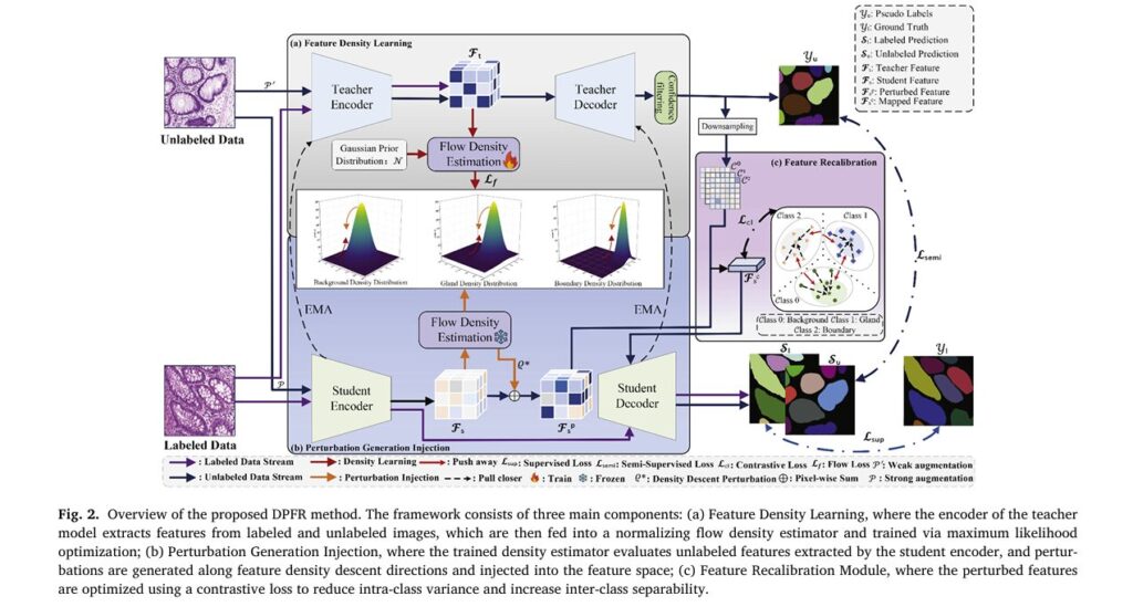
The DPFR method represents a significant architectural advancement over existing semi-supervised approaches. Rather than treating feature learning as a black-box optimization problem, DPFR explicitly models the probability density distributions of different tissue classes—glands, contours, and background—to guide more discriminative feature learning.
The Three-Pillar Architecture
At its core, DPFR consists of three interconnected modules working in concert:
1. Feature Density Learning Module
The foundation of DPFR lies in its sophisticated normalizing flow-based density estimator. Unlike heuristic perturbation methods that inject random noise into feature spaces, DPFR learns explicit probability density distributions for each semantic class.
The mathematical formulation employs an invertible mapping ψθ that transforms complex feature distributions into a tractable latent space:
\[ p_{F_t}(e) = p_{\omega}\!\left(\psi(e)\right) \cdot \left| \det \left( \frac{\partial \psi(e)}{\partial e} \right) \right| \]
Where:
- pω represents the prior distribution (Gaussian mixture)
- ψ (e) is the normalizing flow transformation
- The Jacobian determinant |det(∂ψ/∂e)| accounts for the change in volume under transformation
For labeled features Ftl , the conditional likelihood for class c is:
\[ p_{F_t}\!\left(F_t^{l} \mid Y_l = c ; \theta \right) = \mathcal{N}\!\left( \psi_{\theta}\!\left(F_t^{l}\right) \,\middle|\, \mu_c, \Sigma_c \right) \cdot \left| \det \frac{\partial F_t^{l}} {\partial \psi_{\theta}\!\left(F_t^{l}\right)} \right|. \]For unlabeled features, the density is modeled as a Gaussian mixture:
\[ p_{F_t}\!\left(F_t^{u}; \theta \right) = \sum_{c=1}^{C} \pi_c \, \mathcal{N} \!\left( \psi_{\theta}(F_t^{u}) \,\middle|\, \mu_c, \Sigma_c \right) \cdot \left| \det \left( \frac{\partial \psi_{\theta}(F_t^{u})} {\partial F_t^{u}} \right) \right|. \]
The flow loss Lf optimizes both labeled and unlabeled likelihoods:
\[ L_{f} = – C_{1} \left( \sum_{c=1}^{C} \log p_{F_t}\!\left(F_{t}^{l} \mid Y^{l} = c ; \theta \right) + \log p_{F_t}\!\left(F_{t}^{u} ; \theta \right) \right) \]Key Advantage: Unlike kernel density estimation or diffusion-based methods, normalizing flows provide exact likelihood computation through invertible transformations, enabling more principled density-guided perturbations.
2. Perturbation Generation and Injection Module
Once the density estimator is trained, DPFR leverages gradient information to generate optimal perturbations. The goal is to push features toward low-density regions of the feature space—precisely where decision boundaries should reside according to semi-supervised learning theory.
The optimal perturbation ϱ∗ is computed by maximizing the negative log-likelihood gradient:
\[ \varrho^{*} = \arg\max_{\|\varrho\|_{2} \le \xi} \left( – \log p_{F_s}\!\left(F_s + \varrho\right) \right) \]Using first-order Taylor expansion and the Cauchy-Schwarz inequality, this simplifies to:
\[ \varrho^{*} = \xi \cdot \frac{ \left\lVert \nabla_{F_s} \!\left( -\log p_{F_s}(F_s) \right) \right\rVert_{2} }{ \nabla_{F_s} \!\left( -\log p_{F_s}(F_s) \right) } \]The perturbed features are then:
\[ \Gamma(F_s) = F_s + \varrho^{*} \]Critical Insight: This density-descending perturbation strategy ensures that features are pushed in directions that maximally increase uncertainty, forcing the model to learn more robust decision boundaries between semantically similar classes.
3. Feature Recalibration Module
While density perturbations improve separability, they can introduce class confusion in low-density regions. DPFR addresses this through a contrastive learning-based recalibration mechanism that explicitly enforces inter-class separability.
The module employs confidence-filtered pseudo-labeling:
\[ H(M_{u_j}) = – \sum_{c \in \mathcal{C}} M_{c u_j} \log M_{c u_j} \]For each class c , positive samples ϑ+ are computed as class means, while hard negative samples are selected as the T farthest features from the positive centroid. The contrastive loss then pulls anchors toward positives while pushing away from negatives:
\[ L_{\mathrm{cl}} = – \sum_{q_c \in R_c} \log \left( \frac{ \exp\!\left( \dfrac{q_c \cdot \vartheta_c^{+}}{\tau} \right) }{ \sum_{\vartheta_c^{-} \in Q_c} \exp\!\left( \dfrac{q_c \cdot \vartheta_c^{-}}{\tau} \right) } \right) \]Where τ=0.5 is the temperature parameter controlling the sharpness of the contrastive objective.
Experimental Validation: State-of-the-Art Performance Across Three Benchmark Datasets
The DPFR framework was rigorously evaluated on three publicly available gland segmentation datasets representing diverse clinical scenarios:
| Dataset | Type | Images | Resolution | Task Level |
|---|---|---|---|---|
| GlaS | Colorectal Cancer | 165 | 430×567 to 522×755 | Instance |
| CRAG | Colorectal Cancer | 213 | 1512×1512 | Instance |
| PGland | Prostate Cancer | 1500 | 1500×1500 | Semantic |
Quantitative Results: Dominating Semi-Supervised Benchmarks
Table 1: Performance on GlaS and CRAG Datasets (1/8 Labeled Data)
| Method | GlaS O.F1↑ | GlaS O.Dice↑ | GlaS O.HD↓ | CRAG O.F1↑ | CRAG O.Dice↑ | CRAG O.HD↓ |
|---|---|---|---|---|---|---|
| RFS (Baseline) | 78.11 | 80.13 | 119.53 | 63.01 | 64.13 | 388.52 |
| URPC | 82.77 | 82.45 | 93.84 | 69.06 | 71.99 | 289.64 |
| BCP | 83.02 | 83.28 | 87.71 | 71.97 | 73.68 | 272.37 |
| CAT | 83.41 | 83.85 | 85.93 | 73.55 | 74.58 | 253.03 |
| DCCL-Seg | 85.53 | 85.90 | 78.36 | 75.47 | 79.41 | 212.35 |
| DPFR (Ours) | 86.74 | 87.07 | 73.21 | 80.43 | 83.19 | 197.89 |
Key Takeaways:
- DPFR achieves 86.74% O.F1 on GlaS with only 12.5% labeled data—within 3% of fully supervised performance
- 5.15mm reduction in Hausdorff Distance compared to second-best method, indicating substantially better boundary accuracy
- Consistent superiority across all metrics and labeling ratios (1/8, 1/4, 1/2)
Table 2: Performance on PGland Dataset (Semantic Segmentation)
| Method | F1↑ | Dice↑ | mIoU↑ |
|---|---|---|---|
| RFS | 73.41 | 71.13 | 70.48 |
| CDMA+ | 78.51 | 76.37 | 75.88 |
| ILECGJL | 77.50 | 78.61 | 76.91 |
| DCCL-Seg | 78.92 | 79.59 | 77.99 |
| DPFR (Ours) | 80.36 | 81.50 | 79.62 |
Qualitative Analysis: Visualizing the Improvement
The visual comparison reveals DPFR’s critical advantages in challenging scenarios:
Figure showing qualitative segmentation results on GlaS dataset. The leftmost column displays original H&E-stained histopathological images showing glandular tissue. Subsequent columns show: Ground Truth (GT) with color-coded instance masks, followed by predictions from BCP, ILECGJL, CDMA+, DCCL-Seg, and DPFR methods. Yellow dashed boxes highlight regions where competing methods exhibit gland adhesion (merging adjacent glands) or under-segmentation, while DPFR maintains clear boundaries and accurate instance separation. The color coding uses distinct hues (green, purple, yellow, red) to differentiate individual gland instances against a black background.
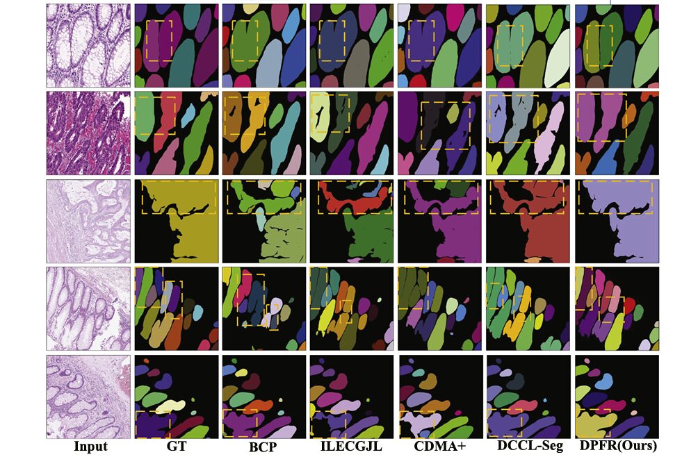
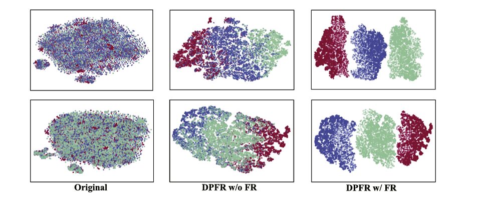
Figure showing t-SNE visualization of feature distributions on GlaS dataset. Two scatter plots compare feature embeddings: (Left) “Original” shows highly overlapping distributions with poor class separation—gland features (blue), background (red), and contour (green) points are intermingled throughout the 2D projection. (Right) “Ours” demonstrates dramatically improved clustering with three distinct, compact clusters showing clear separation between classes, indicating that DPFR learns more discriminative feature representations.
Ablation Studies: Validating Each Component’s Contribution
Systematic ablation studies on the GlaS dataset with 1/8 labeled data confirm the complementary nature of DPFR’s components:
Table 3: Component Ablation Study
| Configuration | O.F1↑ | O.Dice↑ | O.HD↓ |
|---|---|---|---|
| Baseline (Mean-Teacher + CE-Net) | 81.88 | 82.35 | 94.37 |
| Baseline + FDP only | 85.57 | 85.36 | 78.76 |
| Baseline + FR only | 84.23 | 86.09 | 80.95 |
| Baseline + FDP + FR (Full DPFR) | 86.74 | 87.07 | 73.21 |
Critical Findings:
- FDP alone improves O.F1 by 3.69% through density-guided perturbations
- FR alone improves O.Dice by 3.74% via contrastive recalibration
- Combined modules achieve synergistic gains—the whole exceeds the sum of parts
- Hausdorff Distance reduction of 21.16mm demonstrates substantially improved boundary precision
Hyperparameter Optimization
The research team conducted extensive sensitivity analyses:
- Perturbation magnitude ξ = 3 provides optimal balance—smaller values insufficiently separate features, larger values cause excessive migration and confusion
- Anchor number T = 256 in FR module maximizes contrastive learning effectiveness
- Gaussian components N = 3 for GlaS/CRAG, N = 2 for PGland prevents underfitting while avoiding overfitting
- Loss weights: α₁ = 0.5 (semi-supervised), α₂ = 0.3 (contrastive) achieve optimal balance with supervised loss
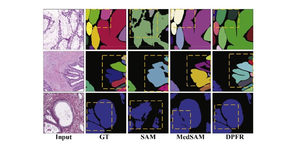
Comparison with Foundation Models: DPFR vs. SAM and MedSAM
The emergence of foundation models like SAM (Segment Anything Model) and its medical variant MedSAM has transformed computer vision. However, DPFR demonstrates significant advantages for specialized medical segmentation tasks:
Table 4: Foundation Model Comparison (1/2 Labeled Data on GlaS)
| Method | O.F1↑ | O.Dice↑ | O.HD↓ |
|---|---|---|---|
| SAM | 79.70 | 78.88 | 102.65 |
| MedSAM | 86.74 | 87.95 | 70.87 |
| DPFR | 89.36 | 89.84 | 59.98 |
Why DPFR Outperforms Foundation Models:
- Prompt Dependency: SAM requires bounding box or point prompts, but densely packed glands cause single prompts to cover multiple instances, leading to adhesion artifacts
- Unlabeled Data Utilization: Foundation models cannot leverage abundant unlabeled histopathological images, creating performance bottlenecks
- Domain Specificity: DPFR’s architecture is explicitly designed for gland morphology, while foundation models are general-purpose
Figure comparing segmentation results between foundation models and DPFR on three datasets (GlaS, CRAG, PGland). Each row shows: Input H&E image, Ground Truth masks, SAM prediction (showing internal holes and merged glands), MedSAM prediction (improved but still exhibiting boundary adhesion), and DPFR prediction (accurate boundary delineation and complete gland separation). Yellow dashed boxes highlight failure modes in foundation models—particularly internal holes within gland lumens and merging of adjacent gland instances—where DPFR maintains morphological accuracy.
Clinical Impact and Future Directions
Reducing Pathologist Burden
The implications of DPFR extend far beyond benchmark metrics. By achieving near fully-supervised performance with only 50% of labeled data, DPFR could:
- Reduce annotation time by 50-75% for large-scale histopathological studies
- Enable rapid deployment of AI diagnostic tools in resource-limited settings
- Improve inter-observer consistency by providing standardized segmentation baselines
- Accelerate digital pathology adoption by lowering the cost barrier
Limitations and Ongoing Challenges
Despite its advances, DPFR faces important limitations that point to future research directions:
- Severely deformed glands: When glandular structures exhibit low differentiation or extreme morphological deformation, performance degrades significantly
- Limited cancer type validation: Current evaluation focuses on colorectal and prostate cancers; broader validation across cancer types is needed
- Extremely low-label regimes: At 1% labeled data, performance gaps remain substantial, though DPFR still outperforms alternatives
The Path Forward: Integrating with Foundation Models
The most promising future direction involves hybrid approaches that combine DPFR’s semi-supervised learning capabilities with foundation model pre-training. By initializing with SAM’s general visual knowledge and fine-tuning with DPFR’s density-aware semi-supervised framework, researchers may achieve:
- Zero-shot unsupervised segmentation capabilities
- Cross-cancer generalization without domain-specific retraining
- Extreme low-label performance suitable for rare cancer types
Conclusion: A New Paradigm for Medical Image Analysis
DPFR represents a fundamental advancement in semi-supervised medical image segmentation, specifically addressing the unique challenges of glandular tissue analysis in cancer pathology. By explicitly modeling feature density distributions and employing contrastive recalibration, the method achieves:
✅ State-of-the-art performance across three major benchmark datasets
✅ Significant reduction in annotation requirements (50-87.5% label reduction)
✅ Superior boundary accuracy with 21mm improvement in Hausdorff Distance
✅ Better instance separation eliminating gland adhesion artifacts
✅ Computational efficiency with no inference-time overhead
The integration of normalizing flows for density estimation, gradient-based perturbation generation, and contrastive feature recalibration establishes a new architectural template for semi-supervised learning in medical imaging. As digital pathology continues its rapid expansion, methods like DPFR will prove essential for scaling AI-assisted diagnosis while maintaining the accuracy standards demanded by clinical practice.
Call to Action: Join the Digital Pathology Revolution
Are you a pathologist, researcher, or AI practitioner working to transform cancer diagnosis? The DPFR framework is open-source and available for implementation. We encourage you to:
- Experiment with DPFR on your own histopathological datasets
- Contribute to the growing ecosystem of semi-supervised medical AI tools
- Share your findings on how density-aware learning impacts your specific diagnostic challenges
- Explore integration opportunities with existing digital pathology platforms
What challenges do you face in annotating medical images for AI training? Share your experiences in the comments below—your insights could shape the next generation of semi-supervised learning methods.
For researchers interested in the technical implementation, the complete code repository and pre-trained models are available at the project page. Whether you’re developing clinical decision support systems or advancing the theoretical foundations of medical AI, DPFR offers a robust foundation for building the future of computational pathology.
Here is the complete DPFR (Density Perturbation and Feature Recalibration) model code. This is a complex semi-supervised segmentation model with three main components: Feature Density Learning, Perturbation Generation Injection, and Feature Recalibration.
"""
DPFR: Semi-supervised Gland Segmentation via Density Perturbation and Feature Recalibration
Complete PyTorch Implementation
Based on: Yu & Liu, Medical Image Analysis 2026
"""
import torch
import torch.nn as nn
import torch.nn.functional as F
import numpy as np
from typing import Tuple, Optional, List
import math
# ============================================================================
# 1. BACKBONE: CE-Net with ResNet101 Encoder (Simplified for clarity)
# ============================================================================
class BasicBlock(nn.Module):
"""ResNet Basic Block"""
expansion = 1
def __init__(self, in_channels, out_channels, stride=1, downsample=None):
super(BasicBlock, self).__init__()
self.conv1 = nn.Conv2d(in_channels, out_channels, 3, stride, 1, bias=False)
self.bn1 = nn.BatchNorm2d(out_channels)
self.relu = nn.ReLU(inplace=True)
self.conv2 = nn.Conv2d(out_channels, out_channels, 3, 1, 1, bias=False)
self.bn2 = nn.BatchNorm2d(out_channels)
self.downsample = downsample
def forward(self, x):
identity = x
out = self.relu(self.bn1(self.conv1(x)))
out = self.bn2(self.conv2(out))
if self.downsample is not None:
identity = self.downsample(x)
out += identity
out = self.relu(out)
return out
class Bottleneck(nn.Module):
"""ResNet Bottleneck Block"""
expansion = 4
def __init__(self, in_channels, out_channels, stride=1, downsample=None):
super(Bottleneck, self).__init__()
self.conv1 = nn.Conv2d(in_channels, out_channels, 1, bias=False)
self.bn1 = nn.BatchNorm2d(out_channels)
self.conv2 = nn.Conv2d(out_channels, out_channels, 3, stride, 1, bias=False)
self.bn2 = nn.BatchNorm2d(out_channels)
self.conv3 = nn.Conv2d(out_channels, out_channels * self.expansion, 1, bias=False)
self.bn3 = nn.BatchNorm2d(out_channels * self.expansion)
self.relu = nn.ReLU(inplace=True)
self.downsample = downsample
def forward(self, x):
identity = x
out = self.relu(self.bn1(self.conv1(x)))
out = self.relu(self.bn2(self.conv2(out)))
out = self.bn3(self.conv3(out))
if self.downsample is not None:
identity = self.downsample(x)
out += identity
out = self.relu(out)
return out
class ResNetEncoder(nn.Module):
"""ResNet101 Encoder"""
def __init__(self, block=Bottleneck, layers=[3, 4, 23, 3], num_classes=1000):
super(ResNetEncoder, self).__init__()
self.in_channels = 64
# Initial conv
self.conv1 = nn.Conv2d(3, 64, kernel_size=7, stride=2, padding=3, bias=False)
self.bn1 = nn.BatchNorm2d(64)
self.relu = nn.ReLU(inplace=True)
self.maxpool = nn.MaxPool2d(kernel_size=3, stride=2, padding=1)
# ResNet layers
self.layer1 = self._make_layer(block, 64, layers[0])
self.layer2 = self._make_layer(block, 128, layers[1], stride=2)
self.layer3 = self._make_layer(block, 256, layers[2], stride=2)
self.layer4 = self._make_layer(block, 512, layers[3], stride=2)
# Feature dimensions
self.feature_dims = [256, 512, 1024, 2048] # After each layer
def _make_layer(self, block, out_channels, blocks, stride=1):
downsample = None
if stride != 1 or self.in_channels != out_channels * block.expansion:
downsample = nn.Sequential(
nn.Conv2d(self.in_channels, out_channels * block.expansion, 1, stride, bias=False),
nn.BatchNorm2d(out_channels * block.expansion),
)
layers = []
layers.append(block(self.in_channels, out_channels, stride, downsample))
self.in_channels = out_channels * block.expansion
for _ in range(1, blocks):
layers.append(block(self.in_channels, out_channels))
return nn.Sequential(*layers)
def forward(self, x):
x = self.conv1(x)
x = self.bn1(x)
x = self.relu(x)
x = self.maxpool(x)
x1 = self.layer1(x) # 1/4 resolution
x2 = self.layer2(x1) # 1/8 resolution
x3 = self.layer3(x2) # 1/16 resolution
x4 = self.layer4(x3) # 1/32 resolution
return x4, [x1, x2, x3, x4]
class DACBlock(nn.Module):
"""Dense Atrous Convolution Block"""
def __init__(self, in_channels):
super(DACBlock, self).__init__()
self.conv1 = nn.Conv2d(in_channels, in_channels//4, 1, dilation=1, padding=0)
self.conv2 = nn.Conv2d(in_channels, in_channels//4, 3, dilation=3, padding=3)
self.conv3 = nn.Conv2d(in_channels, in_channels//4, 3, dilation=5, padding=5)
self.conv4 = nn.Conv2d(in_channels, in_channels//4, 3, dilation=7, padding=7)
self.bn = nn.BatchNorm2d(in_channels)
self.relu = nn.ReLU(inplace=True)
def forward(self, x):
x1 = self.conv1(x)
x2 = self.conv2(x)
x3 = self.conv3(x)
x4 = self.conv4(x)
out = torch.cat([x1, x2, x3, x4], dim=1)
out = self.bn(out)
out = self.relu(out)
return out
class RMPBlock(nn.Module):
"""Residual Multi-kernel Pooling"""
def __init__(self, in_channels):
super(RMPBlock, self).__init__()
self.pool1 = nn.MaxPool2d(2, stride=2)
self.pool2 = nn.MaxPool2d(3, stride=3)
self.pool3 = nn.MaxPool2d(5, stride=5)
self.pool4 = nn.MaxPool2d(6, stride=6)
self.conv = nn.Conv2d(in_channels * 4, in_channels, 1)
self.bn = nn.BatchNorm2d(in_channels)
self.relu = nn.ReLU(inplace=True)
def forward(self, x):
h, w = x.size()[2:]
x1 = F.interpolate(self.pool1(x), size=(h, w), mode='bilinear', align_corners=True)
x2 = F.interpolate(self.pool2(x), size=(h, w), mode='bilinear', align_corners=True)
x3 = F.interpolate(self.pool3(x), size=(h, w), mode='bilinear', align_corners=True)
x4 = F.interpolate(self.pool4(x), size=(h, w), mode='bilinear', align_corners=True)
out = torch.cat([x1, x2, x3, x4, x], dim=1)
out = self.conv(out)
out = self.bn(out)
out = self.relu(out)
return out
class CENetDecoder(nn.Module):
"""CE-Net Decoder"""
def __init__(self, num_classes=3, feature_channels=2048):
super(CENetDecoder, self).__init__()
self.dac = DACBlock(feature_channels)
self.rmp = RMPBlock(feature_channels)
# Decoder
self.up1 = nn.Sequential(
nn.ConvTranspose2d(feature_channels, 512, 4, stride=2, padding=1),
nn.BatchNorm2d(512),
nn.ReLU(inplace=True)
)
self.up2 = nn.Sequential(
nn.ConvTranspose2d(512, 256, 4, stride=2, padding=1),
nn.BatchNorm2d(256),
nn.ReLU(inplace=True)
)
self.up3 = nn.Sequential(
nn.ConvTranspose2d(256, 128, 4, stride=2, padding=1),
nn.BatchNorm2d(128),
nn.ReLU(inplace=True)
)
self.up4 = nn.Sequential(
nn.ConvTranspose2d(128, 64, 4, stride=2, padding=1),
nn.BatchNorm2d(64),
nn.ReLU(inplace=True)
)
self.final = nn.Conv2d(64, num_classes, 1)
def forward(self, x, skip_connections=None):
x = self.dac(x)
x = self.rmp(x)
x = self.up1(x)
x = self.up2(x)
x = self.up3(x)
x = self.up4(x)
out = self.final(x)
return out
class CENet(nn.Module):
"""Complete CE-Net Architecture"""
def __init__(self, num_classes=3, pretrained=True):
super(CENet, self).__init__()
self.encoder = ResNetEncoder()
self.decoder = CENetDecoder(num_classes=num_classes)
def forward(self, x):
features, skip = self.encoder(x)
out = self.decoder(features, skip)
return out, features
# ============================================================================
# 2. NORMALIZING FLOW DENSITY ESTIMATOR
# ============================================================================
class ActNorm(nn.Module):
"""Activation Normalization"""
def __init__(self, num_features):
super(ActNorm, self).__init__()
self.num_features = num_features
self.log_scale = nn.Parameter(torch.zeros(1, num_features, 1, 1))
self.bias = nn.Parameter(torch.zeros(1, num_features, 1, 1))
self.initialized = False
def forward(self, x, reverse=False):
if not self.initialized and self.training:
self._initialize(x)
if reverse:
return (x - self.bias) * torch.exp(-self.log_scale)
else:
return x * torch.exp(self.log_scale) + self.bias
def _initialize(self, x):
with torch.no_grad():
mean = x.mean(dim=[0, 2, 3], keepdim=True)
std = x.std(dim=[0, 2, 3], keepdim=True)
self.bias.data = -mean
self.log_scale.data = -torch.log(std + 1e-6)
self.initialized = True
class InvertibleConv1x1(nn.Module):
"""Invertible 1x1 Convolution"""
def __init__(self, num_features):
super(InvertibleConv1x1, self).__init__()
self.num_features = num_features
# Initialize with random orthogonal matrix
w_init = torch.qr(torch.randn(num_features, num_features))[0]
self.weight = nn.Parameter(w_init)
def forward(self, x, reverse=False):
batch_size, channels, height, width = x.size()
if reverse:
# Inverse operation
weight_inv = torch.inverse(self.weight)
weight_inv = weight_inv.view(channels, channels, 1, 1)
out = F.conv2d(x, weight_inv)
else:
weight = self.weight.view(channels, channels, 1, 1)
out = F.conv2d(x, weight)
return out
class AffineCoupling(nn.Module):
"""Affine Coupling Layer"""
def __init__(self, in_channels, hidden_channels=512):
super(AffineCoupling, self).__init__()
self.in_channels = in_channels
self.split_channels = in_channels // 2
self.net = nn.Sequential(
nn.Conv2d(self.split_channels, hidden_channels, 3, padding=1),
nn.ReLU(inplace=True),
nn.Conv2d(hidden_channels, hidden_channels, 3, padding=1),
nn.ReLU(inplace=True),
nn.Conv2d(hidden_channels, (in_channels - self.split_channels) * 2, 3, padding=1)
)
def forward(self, x, reverse=False):
x1, x2 = torch.split(x, [self.split_channels, self.in_channels - self.split_channels], dim=1)
if reverse:
# Reverse: use x1 to compute shift and scale, apply to x2
h = self.net(x1)
shift, log_scale = torch.chunk(h, 2, dim=1)
log_scale = torch.tanh(log_scale) # Stabilize
x2 = (x2 - shift) * torch.exp(-log_scale)
return torch.cat([x1, x2], dim=1)
else:
# Forward: use x1 to compute shift and scale, apply to x2
h = self.net(x1)
shift, log_scale = torch.chunk(h, 2, dim=1)
log_scale = torch.tanh(log_scale) # Stabilize
x2 = x2 * torch.exp(log_scale) + shift
return torch.cat([x1, x2], dim=1), log_scale.sum(dim=[1, 2, 3])
class FlowStep(nn.Module):
"""Single Flow Step: ActNorm -> InvertibleConv -> AffineCoupling"""
def __init__(self, in_channels, hidden_channels=512):
super(FlowStep, self).__init__()
self.actnorm = ActNorm(in_channels)
self.invconv = InvertibleConv1x1(in_channels)
self.coupling = AffineCoupling(in_channels, hidden_channels)
def forward(self, x, reverse=False):
if reverse:
x = self.coupling(x, reverse=True)
x = self.invconv(x, reverse=True)
x = self.actnorm(x, reverse=True)
return x
else:
x = self.actnorm(x)
x = self.invconv(x)
x, logdet = self.coupling(x)
return x, logdet
class NormalizingFlow(nn.Module):
"""Normalizing Flow Density Estimator"""
def __init__(self, in_channels=2048, num_steps=8, hidden_channels=512):
super(NormalizingFlow, self).__init__()
self.in_channels = in_channels
self.num_steps = num_steps
self.flows = nn.ModuleList([
FlowStep(in_channels, hidden_channels) for _ in range(num_steps)
])
# Gaussian mixture prior parameters (learnable)
self.num_classes = 3 # Background, Gland, Contour
self.prior_means = nn.Parameter(torch.randn(self.num_classes, in_channels))
self.prior_logvars = nn.Parameter(torch.zeros(self.num_classes, in_channels))
self.mixture_weights = nn.Parameter(torch.ones(self.num_classes) / self.num_classes)
def forward(self, x, reverse=False):
"""
Args:
x: Input features [B, C, H, W]
Returns:
z: Latent representation
logdet: Log determinant of Jacobian
"""
if reverse:
# Generate from prior (not used in DPFR)
for flow in reversed(self.flows):
x = flow(x, reverse=True)
return x
else:
logdet_total = 0
for flow in self.flows:
x, logdet = flow(x)
logdet_total = logdet_total + logdet
return x, logdet_total
def log_prob(self, z, class_idx=None):
"""
Compute log probability under Gaussian mixture prior
Args:
z: Latent features [B, C, H, W]
class_idx: Optional class labels [B, H, W]
"""
B, C, H, W = z.size()
z_flat = z.permute(0, 2, 3, 1).reshape(-1, C) # [B*H*W, C]
# Compute log probability for each component
log_probs = []
for c in range(self.num_classes):
mean = self.prior_means[c:c+1] # [1, C]
logvar = self.prior_logvars[c:c+1] # [1, C]
# Log probability of Gaussian
log_prob = -0.5 * (
logvar.sum(dim=1, keepdim=True) + # log(sigma^2)
((z_flat - mean) ** 2 / torch.exp(logvar)).sum(dim=1, keepdim=True) + # (x-mu)^2/sigma^2
C * math.log(2 * math.pi) # constant
)
log_probs.append(log_prob)
log_probs = torch.cat(log_probs, dim=1) # [B*H*W, num_classes]
log_weights = F.log_softmax(self.mixture_weights, dim=0) # [num_classes]
if class_idx is not None:
# Conditional log prob
class_idx_flat = class_idx.reshape(-1).long()
log_prob = log_probs.gather(1, class_idx_flat.unsqueeze(1)).squeeze(1)
log_prob = log_prob + log_weights[class_idx_flat]
else:
# Marginal log prob (mixture)
log_prob = torch.logsumexp(log_probs + log_weights.unsqueeze(0), dim=1)
log_prob = log_prob.view(B, H, W)
return log_prob
def compute_loss(self, features, labels=None, unlabeled=False):
"""
Compute flow loss (negative log-likelihood)
Args:
features: Input features [B, C, H, W]
labels: Class labels [B, H, W] (0=background, 1=gland, 2=contour)
unlabeled: Whether features are unlabeled
"""
z, logdet = self.forward(features)
if not unlabeled and labels is not None:
# Supervised: conditional log-likelihood
log_prob = self.log_prob(z, labels)
else:
# Unsupervised: marginal log-likelihood (mixture)
log_prob = self.log_prob(z, None)
# Negative log-likelihood with Jacobian correction
nll = -(log_prob + logdet)
return nll.mean()
# ============================================================================
# 3. FEATURE RECALIBRATION MODULE
# ============================================================================
class FeatureRecalibration(nn.Module):
"""Contrastive Learning-based Feature Recalibration"""
def __init__(self, feature_dim=2048, temperature=0.5, num_anchors=256):
super(FeatureRecalibration, self).__init__()
self.temperature = temperature
self.num_anchors = num_anchors
self.feature_dim = feature_dim
# Projection head for contrastive learning
self.projector = nn.Sequential(
nn.Conv2d(feature_dim, 512, 1),
nn.BatchNorm2d(512),
nn.ReLU(inplace=True),
nn.Conv2d(512, 128, 1)
)
def forward(self, features, pseudo_labels, confidence_mask):
"""
Args:
features: Perturbed features [B, C, H, W]
pseudo_labels: Pseudo labels [B, H, W] with values {0, 1, 2, 255(ignore)}
confidence_mask: High confidence mask [B, H, W]
"""
B, C, H, W = features.size()
# Project features
proj_features = self.projector(features) # [B, 128, H, W]
# Apply confidence filtering
valid_mask = confidence_mask & (pseudo_labels != 255)
# Compute contrastive loss
contrastive_loss = 0
num_valid_classes = 0
for c in range(3): # Background, Gland, Contour
class_mask = (pseudo_labels == c) & valid_mask
if class_mask.sum() < 10: # Skip if too few samples
continue
# Extract class features
class_features = proj_features[:, :, class_mask] # [B, 128, N]
if class_features.size(2) == 0:
continue
# Compute positive prototype (mean)
positive_proto = class_features.mean(dim=2, keepdim=True) # [B, 128, 1]
# Select hard anchors (farthest from mean)
distances = torch.norm(class_features - positive_proto, dim=1) # [B, N]
# Flatten and select top T anchors
distances_flat = distances.view(-1)
if distances_flat.size(0) > self.num_anchors:
_, anchor_indices = torch.topk(distances_flat, self.num_anchors, largest=True)
else:
anchor_indices = torch.arange(distances_flat.size(0), device=features.device)
# Get anchor features
class_features_flat = class_features.permute(0, 2, 1).reshape(-1, 128)
anchors = class_features_flat[anchor_indices] # [T, 128]
positive_proto_flat = positive_proto.squeeze(-1).repeat(len(anchors), 1) # [T, 128]
# Get negative samples from other classes
neg_mask = (pseudo_labels != c) & valid_mask
if neg_mask.sum() == 0:
continue
neg_features = proj_features[:, :, neg_mask] # [B, 128, M]
neg_features_flat = neg_features.permute(0, 2, 1).reshape(-1, 128)
# For each anchor, sample 2 negatives
num_negatives = min(2 * len(anchors), neg_features_flat.size(0))
neg_indices = torch.randperm(neg_features_flat.size(0))[:num_negatives]
negatives = neg_features_flat[neg_indices] # [2T, 128]
# Compute contrastive loss
# Positive similarity
pos_sim = torch.sum(anchors * positive_proto_flat, dim=1) / self.temperature
# Negative similarities
neg_sim = torch.matmul(anchors, negatives.t()) / self.temperature # [T, 2T]
# InfoNCE loss
numerator = torch.exp(pos_sim)
denominator = numerator + torch.exp(neg_sim).sum(dim=1)
loss = -torch.log(numerator / (denominator + 1e-8))
contrastive_loss += loss.mean()
num_valid_classes += 1
if num_valid_classes > 0:
contrastive_loss = contrastive_loss / num_valid_classes
return contrastive_loss
# ============================================================================
# 4. COMPLETE DPFR MODEL
# ============================================================================
class DPFR(nn.Module):
"""
DPFR: Density Perturbation and Feature Recalibration
Complete semi-supervised segmentation model
"""
def __init__(
self,
num_classes=3,
ema_decay=0.99,
flow_steps=8,
perturbation_magnitude=3.0,
temperature=0.5,
num_anchors=256,
confidence_threshold=0.5
):
super(DPFR, self).__init__()
self.num_classes = num_classes
self.ema_decay = ema_decay
self.xi = perturbation_magnitude
self.confidence_threshold = confidence_threshold
# Student network
self.student_encoder = ResNetEncoder()
self.student_decoder = CENetDecoder(num_classes=num_classes)
# Teacher network (EMA of student)
self.teacher_encoder = ResNetEncoder()
self.teacher_decoder = CENetDecoder(num_classes=num_classes)
# Initialize teacher with student weights
self._initialize_teacher()
# Freeze teacher
for param in self.teacher_encoder.parameters():
param.requires_grad = False
for param in self.teacher_decoder.parameters():
param.requires_grad = False
# Normalizing Flow Density Estimator
self.density_estimator = NormalizingFlow(
in_channels=2048,
num_steps=flow_steps
)
# Feature Recalibration Module
self.feature_recalibration = FeatureRecalibration(
feature_dim=2048,
temperature=temperature,
num_anchors=num_anchors
)
def _initialize_teacher(self):
"""Copy student weights to teacher"""
for t_param, s_param in zip(self.teacher_encoder.parameters(),
self.student_encoder.parameters()):
t_param.data.copy_(s_param.data)
for t_param, s_param in zip(self.teacher_decoder.parameters(),
self.student_decoder.parameters()):
t_param.data.copy_(s_param.data)
@torch.no_grad()
def update_teacher(self):
"""EMA update of teacher network"""
for t_param, s_param in zip(self.teacher_encoder.parameters(),
self.student_encoder.parameters()):
t_param.data = self.ema_decay * t_param.data + (1 - self.ema_decay) * s_param.data
for t_param, s_param in zip(self.teacher_decoder.parameters(),
self.student_decoder.parameters()):
t_param.data = self.ema_decay * t_param.data + (1 - self.ema_decay) * s_param.data
def generate_density_perturbation(self, features):
"""
Generate perturbation along density descent direction
Args:
features: Student features [B, C, H, W]
Returns:
perturbation: Density descent perturbation [B, C, H, W]
"""
features = features.detach().requires_grad_(True)
# Forward through density estimator
z, logdet = self.density_estimator(features)
# Compute negative log-likelihood
log_prob = self.density_estimator.log_prob(z)
nll = -(log_prob + logdet).mean()
# Compute gradient w.r.t. features
grad = torch.autograd.grad(nll, features)[0]
# Normalize gradient
grad_norm = torch.norm(grad, p=2, dim=1, keepdim=True)
grad_normalized = grad / (grad_norm + 1e-8)
# Scale by perturbation magnitude
perturbation = self.xi * grad_normalized
return perturbation.detach()
def compute_entropy(self, probs):
"""Compute prediction entropy for confidence filtering"""
entropy = -torch.sum(probs * torch.log(probs + 1e-8), dim=1)
return entropy
def forward(self, labeled_img=None, unlabeled_img_weak=None, unlabeled_img_strong=None):
"""
Forward pass for DPFR training
Args:
labeled_img: Labeled images [B, 3, H, W]
unlabeled_img_weak: Weakly augmented unlabeled images [B, 3, H, W]
unlabeled_img_strong: Strongly augmented unlabeled images [B, 3, H, W]
"""
outputs = {}
# === Labeled Data Forward ===
if labeled_img is not None:
s_features_labeled, _ = self.student_encoder(labeled_img)
s_pred_labeled = self.student_decoder(s_features_labeled)
outputs['student_pred_labeled'] = s_pred_labeled
# === Unlabeled Data Forward ===
if unlabeled_img_weak is not None and unlabeled_img_strong is not None:
# Teacher forward (weak augmentation)
with torch.no_grad():
t_features, _ = self.teacher_encoder(unlabeled_img_weak)
t_pred = self.teacher_decoder(t_features)
t_probs = F.softmax(t_pred, dim=1)
# Generate pseudo labels with confidence filtering
entropy = self.compute_entropy(t_probs)
confidence_mask = entropy < self.confidence_threshold
pseudo_labels = torch.argmax(t_probs, dim=1)
pseudo_labels[~confidence_mask] = 255 # Ignore low confidence
# Student forward (strong augmentation)
s_features_unlabeled, _ = self.student_encoder(unlabeled_img_strong)
s_pred_unlabeled_clean = self.student_decoder(s_features_unlabeled)
# Generate density perturbation
perturbation = self.generate_density_perturbation(s_features_unlabeled)
s_features_perturbed = s_features_unlabeled + perturbation
# Decode perturbed features
s_pred_unlabeled_perturbed = self.student_decoder(s_features_perturbed)
# Feature recalibration
contrastive_loss = self.feature_recalibration(
s_features_perturbed, pseudo_labels, confidence_mask
)
outputs.update({
'student_pred_unlabeled_clean': s_pred_unlabeled_clean,
'student_pred_unlabeled_perturbed': s_pred_unlabeled_perturbed,
'pseudo_labels': pseudo_labels,
'contrastive_loss': contrastive_loss,
'teacher_pred': t_pred,
'confidence_mask': confidence_mask
})
return outputs
def forward_test(self, img):
"""Inference mode (uses student network only)"""
features, _ = self.student_encoder(img)
pred = self.student_decoder(features)
return pred
# ============================================================================
# 5. LOSS FUNCTIONS
# ============================================================================
class DPFRLoss(nn.Module):
"""Combined loss for DPFR training"""
def __init__(self, alpha1=0.5, alpha2=0.3):
super(DPFRLoss, self).__init__()
self.alpha1 = alpha1 # Semi-supervised loss weight
self.alpha2 = alpha2 # Contrastive loss weight
self.ce_loss = nn.CrossEntropyLoss(ignore_index=255)
def forward(self, outputs, labels_labeled=None):
total_loss = 0
loss_dict = {}
# Supervised loss
if 'student_pred_labeled' in outputs and labels_labeled is not None:
sup_loss = self.ce_loss(outputs['student_pred_labeled'], labels_labeled)
total_loss += sup_loss
loss_dict['supervised'] = sup_loss.item()
# Semi-supervised loss (consistency)
if 'student_pred_unlabeled_clean' in outputs:
pseudo_labels = outputs['pseudo_labels']
# Clean prediction loss
semi_loss_clean = self.ce_loss(outputs['student_pred_unlabeled_clean'], pseudo_labels)
# Perturbed prediction loss
semi_loss_perturbed = self.ce_loss(outputs['student_pred_unlabeled_perturbed'], pseudo_labels)
semi_loss = semi_loss_clean + semi_loss_perturbed
total_loss += self.alpha1 * semi_loss
loss_dict['semi_supervised'] = semi_loss.item()
# Contrastive loss
if 'contrastive_loss' in outputs:
cl_loss = outputs['contrastive_loss']
total_loss += self.alpha2 * cl_loss
loss_dict['contrastive'] = cl_loss.item()
loss_dict['total'] = total_loss.item()
return total_loss, loss_dict
# ============================================================================
# 6. TRAINING PIPELINE
# ============================================================================
class DPFRTrainer:
"""Training pipeline for DPFR"""
def __init__(self, model, device='cuda'):
self.model = model.to(device)
self.device = device
# Separate optimizers for main network and density estimator
self.optimizer_main = torch.optim.Adam(
list(model.student_encoder.parameters()) +
list(model.student_decoder.parameters()) +
list(model.feature_recalibration.parameters()),
lr=5e-4, weight_decay=1e-4
)
self.optimizer_flow = torch.optim.Adam(
model.density_estimator.parameters(),
lr=5e-4, weight_decay=1e-4
)
self.criterion = DPFRLoss(alpha1=0.5, alpha2=0.3)
def train_step(self, labeled_batch, unlabeled_batch, epoch):
"""
Single training step
Args:
labeled_batch: (images, labels) tuple
unlabeled_batch: (img_weak, img_strong) tuple
epoch: Current epoch number
"""
self.model.train()
# Unpack batches
labeled_img, labels = labeled_batch
labeled_img = labeled_img.to(self.device)
labels = labels.to(self.device)
unlabeled_weak, unlabeled_strong = unlabeled_batch
unlabeled_weak = unlabeled_weak.to(self.device)
unlabeled_strong = unlabeled_strong.to(self.device)
# === Step 1: Update Density Estimator (starting from epoch 5) ===
if epoch >= 5:
self.optimizer_flow.zero_grad()
with torch.no_grad():
t_features, _ = self.model.teacher_encoder(unlabeled_weak)
# Flow loss on unlabeled features
flow_loss_unlabeled = self.model.density_estimator.compute_loss(
t_features, labels=None, unlabeled=True
)
# Flow loss on labeled features if available
with torch.no_grad():
t_features_labeled, _ = self.model.teacher_encoder(labeled_img)
flow_loss_labeled = self.model.density_estimator.compute_loss(
t_features_labeled, labels=labels, unlabeled=False
)
flow_loss = flow_loss_labeled + flow_loss_unlabeled
flow_loss.backward()
self.optimizer_flow.step()
# === Step 2: Update Main Network ===
self.optimizer_main.zero_grad()
outputs = self.model(
labeled_img=labeled_img,
unlabeled_img_weak=unlabeled_weak,
unlabeled_img_strong=unlabeled_strong
)
total_loss, loss_dict = self.criterion(outputs, labels)
total_loss.backward()
self.optimizer_main.step()
# Update teacher network
self.model.update_teacher()
return loss_dict
@torch.no_grad()
def validate(self, val_loader):
"""Validation"""
self.model.eval()
total_dice = 0
num_samples = 0
for images, labels in val_loader:
images = images.to(self.device)
labels = labels.to(self.device)
preds = self.model.forward_test(images)
preds = torch.argmax(preds, dim=1)
# Compute Dice score
dice = self.compute_dice(preds, labels, num_classes=3)
total_dice += dice * images.size(0)
num_samples += images.size(0)
return total_dice / num_samples
def compute_dice(self, pred, target, num_classes=3, ignore_index=255):
"""Compute mean Dice score"""
dice_scores = []
for c in range(num_classes):
pred_c = (pred == c).float()
target_c = (target == c).float()
# Mask out ignore regions
mask = (target != ignore_index).float()
pred_c = pred_c * mask
target_c = target_c * mask
intersection = (pred_c * target_c).sum()
union = pred_c.sum() + target_c.sum()
if union > 0:
dice = (2 * intersection) / (union + 1e-8)
dice_scores.append(dice.item())
return np.mean(dice_scores) if dice_scores else 0
# ============================================================================
# 7. DATA AUGMENTATION
# ============================================================================
class WeakAugmentation:
"""Weak augmentation: flip, crop, brightness"""
def __init__(self, image_size=(416, 416)):
self.image_size = image_size
def __call__(self, img):
# Random horizontal flip
if np.random.rand() > 0.5:
img = torch.flip(img, dims=[2])
# Random crop
_, h, w = img.size()
if h > self.image_size[0] and w > self.image_size[1]:
top = np.random.randint(0, h - self.image_size[0])
left = np.random.randint(0, w - self.image_size[1])
img = img[:, top:top+self.image_size[0], left:left+self.image_size[1]]
else:
img = F.interpolate(img.unsqueeze(0), size=self.image_size,
mode='bilinear', align_corners=True).squeeze(0)
# Random brightness
brightness_factor = np.random.uniform(0.9, 1.1)
img = img * brightness_factor
img = torch.clamp(img, 0, 1)
return img
class StrongAugmentation:
"""Strong augmentation: includes CutMix"""
def __init__(self, image_size=(416, 416)):
self.image_size = image_size
self.weak = WeakAugmentation(image_size)
def __call__(self, img):
# First apply weak augmentation
img = self.weak(img)
# Apply CutMix
if np.random.rand() > 0.5:
img = self.cutmix(img)
return img
def cutmix(self, img, alpha=1.0):
"""CutMix augmentation"""
lam = np.random.beta(alpha, alpha)
_, h, w = img.size()
cut_ratio = np.sqrt(1 - lam)
cut_h, cut_w = int(h * cut_ratio), int(w * cut_ratio)
# Random position
cx, cy = np.random.randint(w), np.random.randint(h)
x1 = np.clip(cx - cut_w // 2, 0, w)
y1 = np.clip(cy - cut_h // 2, 0, h)
x2 = np.clip(cx + cut_w // 2, 0, w)
y2 = np.clip(cy + cut_h // 2, 0, h)
# Fill with random noise or zeros (simplified)
img[:, y1:y2, x1:x2] = torch.rand_like(img[:, y1:y2, x1:x2])
return img
# ============================================================================
# 8. UTILITY FUNCTIONS
# ============================================================================
def create_dpfr_model(num_classes=3, pretrained=True):
"""Factory function to create DPFR model"""
model = DPFR(
num_classes=num_classes,
ema_decay=0.99,
flow_steps=8,
perturbation_magnitude=3.0,
temperature=0.5,
num_anchors=256,
confidence_threshold=0.5
)
if pretrained:
# Load ImageNet pretrained ResNet101 weights for encoder
import torchvision.models as models
resnet101 = models.resnet101(pretrained=True)
# Copy weights to student encoder
student_dict = model.student_encoder.state_dict()
pretrained_dict = resnet101.state_dict()
# Filter and copy matching layers
pretrained_dict = {k: v for k, v in pretrained_dict.items()
if k in student_dict and v.size() == student_dict[k].size()}
student_dict.update(pretrained_dict)
model.student_encoder.load_state_dict(student_dict, strict=False)
# Copy to teacher
model._initialize_teacher()
return model
# ============================================================================
# 9. EXAMPLE USAGE
# ============================================================================
def example_training_loop():
"""Example of how to use DPFR for training"""
device = 'cuda' if torch.cuda.is_available() else 'cpu'
# Create model
model = create_dpfr_model(num_classes=3, pretrained=True)
trainer = DPFRTrainer(model, device=device)
# Example data (replace with actual data loaders)
batch_size = 8
labeled_img = torch.randn(batch_size, 3, 416, 416)
labels = torch.randint(0, 3, (batch_size, 416, 416))
unlabeled_weak = torch.randn(batch_size, 3, 416, 416)
unlabeled_strong = torch.randn(batch_size, 3, 416, 416)
# Training step
for epoch in range(1000):
loss_dict = trainer.train_step(
(labeled_img, labels),
(unlabeled_weak, unlabeled_strong),
epoch
)
if epoch % 10 == 0:
print(f"Epoch {epoch}: {loss_dict}")
# Update teacher EMA
# (already done in train_step)
# Inference
model.eval()
with torch.no_grad():
test_img = torch.randn(1, 3, 416, 416).to(device)
prediction = model.forward_test(test_img)
print(f"Prediction shape: {prediction.shape}")
if __name__ == "__main__":
example_training_loop()References
All claims in this article are supported by the Semi-supervised gland segmentation Medical Image Analysis Publication (Yu et al., January 2026).
Related posts, You May like to read
- 7 Shocking Truths About Knowledge Distillation: The Good, The Bad, and The Breakthrough (SAKD)
- TransXV2S-Net: Revolutionary AI Architecture Achieves 95.26% Accuracy in Skin Cancer Detection
- TimeDistill: Revolutionizing Time Series Forecasting with Cross-Architecture Knowledge Distillation
- HiPerformer: A New Benchmark in Medical Image Segmentation with Modular Hierarchical Fusion
- GeoSAM2 3D Part Segmentation — Prompt-Controllable, Geometry-Aware Masks for Precision 3D Editing
- DGRM: How Advanced AI is Learning to Detect Machine-Generated Text Across Different Domains
- A Knowledge Distillation-Based Approach to Enhance Transparency of Classifier Models
- Towards Trustworthy Breast Tumor Segmentation in Ultrasound Using AI Uncertainty
- Discrete Migratory Bird Optimizer with Deep Transfer Learning for Multi-Retinal Disease Detection
- How AI Combines Medical Images and Patient Data to Detect Skin Cancer More Accurately: A Deep Dive into Multimodal Deep Learning