Introduction: The Critical Challenge in Breast Cancer Screening
Breast cancer remains the leading cause of cancer-related deaths among women worldwide, accounting for 15.5% of all female cancer fatalities according to 2024 global statistics. With incidence rates rising particularly in low and middle-income regions, the need for accurate, accessible early detection has never been more urgent. While mammography has long served as the cornerstone of breast cancer screening, it faces significant limitations—especially for the 50% of women globally who have dense breast tissue, a figure that exceeds 60-70% in Asian populations.
Handheld ultrasound (HHUS) has emerged as an indispensable complementary tool, offering non-radiative, cost-effective, and real-time imaging capabilities that excel at differentiating cystic from solid masses. However, conventional 2D ultrasound scanning suffers from three critical weaknesses:
Operator-dependent acquisition leading to inconsistent image quality
Subjective 2D interpretation varying significantly between sonographers
Imprecise clock-face annotation complicating longitudinal follow-up
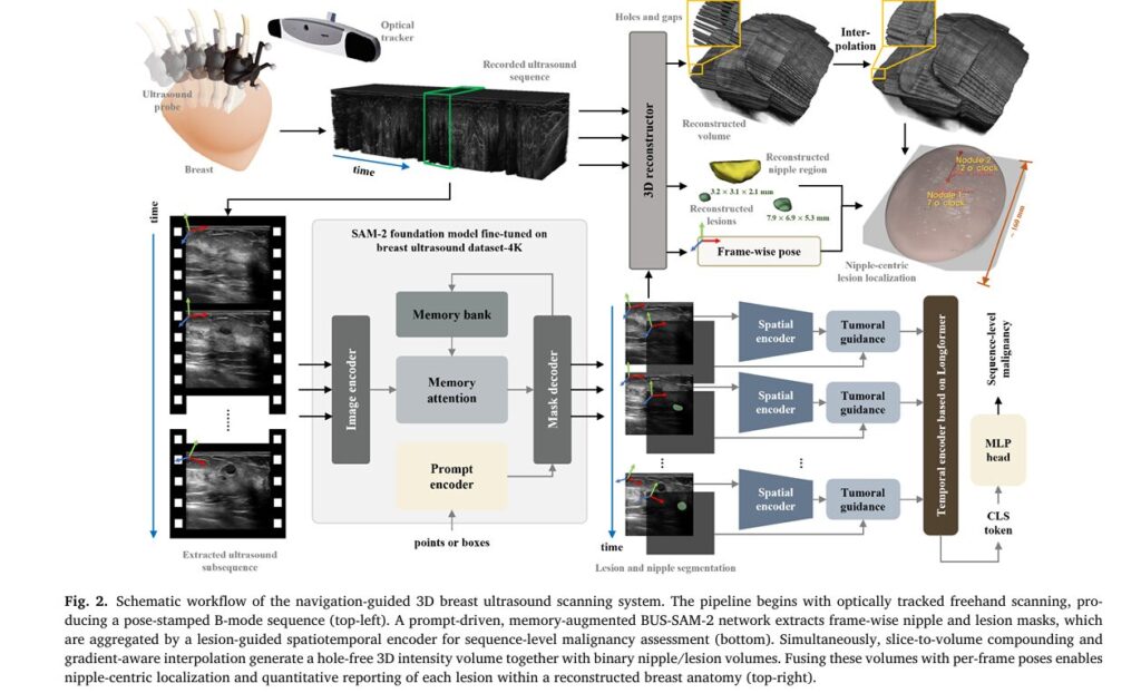
These limitations create serious clinical consequences. Inaccurate lesion localization can lead to enlarged excision volumes, elevated recurrence risks post-surgery, and compromised treatment planning. A groundbreaking study published in Medical Image Analysis (2026) introduces an innovative solution: a navigation-guided 3D breast ultrasound scanning and reconstruction system that seamlessly integrates optical tracking, foundation AI models, and intelligent spatiotemporal analysis.
Understanding the Technology: Core Components of the Navigation-Guided System
The Hardware Architecture
The proposed system represents a sophisticated fusion of clinical ultrasound equipment and precision tracking technology. At its core, the setup comprises three integrated modules:
| Component | Specifications | Function |
|---|---|---|
| Clinical Ultrasound Console | Eagus R9 with L9-3U linear probe (2.5-9.0 MHz, 40mm depth) | High-resolution B-mode imaging |
| Infrared Optical Tracker | Polaris system (NDI), 60Hz maximum frequency | Real-time probe pose tracking |
| Mobile Workstation | Intel Core i9-12900H, 32GB RAM, NVIDIA RTX 3080Ti | Real-time processing and reconstruction |
The optical tracker provides a pyramidal measurement volume extending to 3.0 meters, mounted approximately 1.5 meters from the patient’s breast. This configuration enables comprehensive breast coverage without restricting sonographer movement.
Spatial and Temporal Calibration: The Foundation of Accuracy
Achieving precise 3D reconstruction requires meticulous calibration. The system employs an improved N-wire phantom method to compute the rigid similarity transform TIP that maps image coordinates to probe coordinates:
\[ \mathbf{x}_{t_i} = \mathbf{O}_V^{T} \cdot \mathbf{I}_O^{T} \cdot \mathbf{t}_i \cdot \begin{pmatrix} u f_x \\ u f_y \\ 0 \\ 1 \end{pmatrix} \]Where:
- xti represents the physical coordinate of pixel p(ufx,ufy) at time ti
- IOTti is the time-varying transform from image to optical tracker frame
- OVT is the custom alignment transform to the reconstructed volume
Temporal calibration addresses synchronization between the optical tracker (20Hz) and ultrasound frame-grabber (50fps). By maximizing the cross-correlation function of normalized position sequences, the system achieves temporal alignment with errors below 3.8ms—well under the 40ms threshold that would compromise volume estimation accuracy.
BUS-SAM-2: Fine-Tuned Foundation Model for Lesion Segmentation
The Power of Prompt-Driven Segmentation
Central to the system’s diagnostic capability is BUS-SAM-2 (Breast Ultrasound Segment Anything Model 2), a fine-tuned variant of Meta’s SAM-2 optimized for breast ultrasound imagery. Trained on a curated 4,000-image multi-center dataset spanning Poland, Brazil, Egypt, and China, this foundation model enables precise, prompt-driven segmentation of both nipples and lesions.
The segmentation process operates through a memory-augmented architecture:
\[ S_{i}^{t} = f_{\theta}^{\mathrm{BUS\!-\!SAM\!-\!2}} \!\left( I_{i}^{t},\, C_{t},\, M_{i}^{t-1} \right) \]Where the memory bank M updates via lightweight transformer with streaming attention:
\[ M_{t}^{\,i} = g_{\phi}\!\left( S_{t}^{\,i}, M_{t-1}^{\,i} \right) \]This design maintains temporal coherence without quadratic computational cost, enabling real-time processing across arbitrary-length sequences.
Key Advantages Over Traditional Methods
- Minimal manual intervention: Requires only sparse positive/negative point prompts
- Automatic propagation: Forward and reverse tracking terminates when Dice overlap falls below 0.1 across 3 successive frames
- Subsequence extraction: Isolates clinically relevant segments from continuous scanning
Hybrid Lesion-Informed Spatiotemporal Transformer (HLST)
Mimicking Clinical Decision-Making
The diagnostic intelligence of the system resides in the Hybrid Lesion-informed Spatiotemporal Transformer (HLST), a novel architecture that replicates how experienced radiologists synthesize information across multiple ultrasound frames. Rather than relying on single-image classification—a major limitation of existing computer-aided diagnosis systems—HLST aggregates intra-lesional and peri-lesional dynamics across the entire temporal sequence.
The architecture processes inputs through three stages:
1. Dual-Stream Spatial Encoding Frame-wise representations Fti∈RD are extracted using a CNN-Transformer hybrid, with embeddings selectively aggregated from diagnostically relevant regions while suppressing irrelevant background.
2. Temporal Longformer Processing The sequence of embeddings Fb:b+k−1 ∈ Rk × D is prepended with a learnable classification token τ ∈ RD :
\[ \tilde{F} = \left[ \tau \, ; \, F_{b:b+k-1} \right] \in \mathbb{R}^{(k+1) \times D} \]A Longformer encoder applies sparse-dense attention—combining local windowed attention on frame tokens with global attention on the classification token. This hybrid strategy reduces complexity from O(n2) to O(n) , accommodating clips of arbitrary duration.
3. Malignancy Prediction The contextualized classification embedding zcls feeds into a lightweight MLP, with training supervised by class-balanced focal loss:
\[ L_{\mathrm{cls}} = – \alpha\, y \,(1-\hat{y})^{\gamma}\,\log(\hat{y}) – (1-\alpha)\,(1-y)\,\hat{y}^{\gamma}\,\log(1-\hat{y}) \]This loss adaptively emphasizes hard-to-classify lesions while maintaining robustness against class imbalance common in breast imaging datasets.
Breakthrough Performance Results
| Metric | HLST (Proposed) | Best Alternative | Improvement |
|---|---|---|---|
| Accuracy | 86.1% | 79.6% | +6.5% |
| Precision | 84.9% | 81.3% | +3.6% |
| Recall | 92.7% | 85.7% | +7.0% |
| F1-Score | 88.5% | 83.2% | +5.3% |
| AUC | 86.8% | 82.7% | +4.1% |
Table: Performance comparison on BUV dataset (186 breast ultrasound videos). HLST significantly outperforms TimeSformer, VideoSwin, UniFormerV2, C3D, and SlowFast architectures (p < 0.05).
Automated Nipple-Centric Localization: Eliminating Operator Dependency
Geometry-Adaptive Clock Projection
One of the system’s most clinically valuable innovations is automated standardized spatial annotation without requiring patient-attached fiducials or pre-marked landmarks. The method establishes a breast-specific polar coordinate system through:
Step 1: Craniocaudal Direction Estimation The system requires sonographers to begin with a standardized downward probe motion, enabling computation of the body axis:
\[ V_{nc} = \frac{\kappa}{|T|^{2}} \left( \sum_{i=1}^{\kappa |T|/2} IV_{pt_i} – \sum_{i=\kappa |T|/2 + 1}^{\kappa |T|} IV_{pt_i} \right) \]Step 2: Ellipsoid Fitting for Projection Plane The breast surface is modeled as a flattened ellipsoid with parameters Θe=(χ,a,b,c,α,β,γ) , optimized to minimize geometric error while ensuring all lesion voxels lie within the volume:
\[ \inf_{P_e} \sum_{\nu_{s_i} \in \widetilde{\mathcal{V}}_{s}^{+}} E_2\!\left(\nu_{s_i}; \Theta_e\right) \]Step 3: Clock-Face Orientation Calculation For each lesion li , the clockwise nipple-centric angle is computed as:
\[ \phi_{l}^{\,i} = \frac{\operatorname{atan2}\!\left( \left( \mathbf{V}_{n l}^{\,i\,\prime} \times \tilde{\mathbf{V}}_{n c}^{\,\prime} \right) \cdot \tilde{\mathbf{V}}_{n p}, \; \tilde{\mathbf{V}}_{n c}^{\,\prime} \cdot \mathbf{V}_{n l}^{\,i\,\prime} \right)}{2\pi} \]This yields standardized clock-face positions (1-12 o’clock) comparable across examinations and institutions.
Phantom Validation: Precision Meets Practice
Validation on three breast phantoms (designated H, S, and C) demonstrated exceptional accuracy against CT reference standards:
| Parameter | Correlation (r) | p-value | Median Absolute Error |
|---|---|---|---|
| Distance to nipple | >0.99 | <0.0001 | 0.35 mm |
| 3D lesion size | >0.97 | <0.0001 | 1.17 × 0.70 × 0.83 mm |
| Clock-face angle | 1.00 | <0.0001 | 0.77° |
Table: Phantom study results showing high correlation with CT ground truth across morphological and positional parameters.
The mean Hausdorff distance of 2.39mm and center distance of 0.85mm between ultrasound and CT reconstructions confirm clinical-grade precision. Notably, the system maintains this accuracy across deformable phantoms, with intra-observer CV ≤4.09% and inter-observer ICC ≥0.953—surpassing existing systems by substantial margins.
Clinical Impact and Real-World Performance
Seamless Workflow Integration
The system has been implemented as BreastLesion3DLocalizer, a 3D Slicer extension module designed for routine clinical deployment. Processing efficiency metrics demonstrate practical viability:
- Segmentation speed: 42 frames per second
- Reconstruction speed: 74 frames per second
- Total processing time: ~2 minutes for 2,000-frame sequence (including 15s segmentation, 30s reconstruction, 35s localization)
Clinical Study Outcomes
Evaluation across 43 female patients (86 breasts) at Shanghai Sixth People’s Hospital revealed:
- Median clock-face discrepancy: 0 hours (perfect agreement)
- Mean clock-face discrepancy: 0.51 hours
- 2D size median difference: 0.7mm × 0.6mm
- BI-RADS concordance: 95.65% (threshold ≥4a), 93.48% (threshold ≥4b)
Advantages Over Existing Technologies
Compared to Automated Breast Volume Scanning (ABVS)
| Feature | ABVS | Navigation-Guided HHUS |
|---|---|---|
| Patient comfort | Requires compression | Contact-only scanning |
| Scanning range | Limited field of view | Full breast coverage |
| Examination time | Prolonged | Comparable to routine |
| Cost | High equipment investment | Leverages existing probes |
| Workflow disruption | Requires dedicated room | Integrates seamlessly |
Compared to Conventional Freehand Systems
The proposed system eliminates critical limitations of previous tracked ultrasound approaches:
- No patient-mounted sensors required (unlike Šroubek et al., 2019)
- Arbitrary tracker positioning—no need for bed-parallel alignment
- Adaptive to any breast geometry without anisotropic scaling to generic models
- Fully automated 3D visualization with quantitative morphometrics
Future Directions and Technical Evolution
While current results are clinically compelling, ongoing research targets several enhancement pathways:
Deformation Compensation Integration of RGB-D cameras for real-time breast surface monitoring could enable pixel-wise deformation correction, recovering compression-free anatomy through probe pose adjustment and respiratory compensation.
Marker-less Tracking Foundation models for 6DOF pose estimation (e.g., FoundationPose) may eventually substitute optical trackers, reducing system cost while maintaining sub-millimeter accuracy.
Doppler Integration Extension to 3D power Doppler reconstruction would enable comprehensive vascular assessment, enriching diagnostic information for lesion characterization.
Automated Prompting Concept prompt engineering could eliminate remaining manual intervention in lesion segmentation, progressing toward fully autonomous screening.
Conclusion: A New Standard for Breast Ultrasound
The navigation-guided 3D breast ultrasound system represents a paradigm shift in early cancer detection—transforming operator-dependent 2D imaging into standardized, quantitative, 3D diagnostic intelligence. By achieving 86.1% diagnostic accuracy while eliminating the variability inherent in conventional practice, this technology addresses critical gaps in the breast cancer care continuum.
For healthcare institutions, the system offers:
- Enhanced diagnostic confidence through foundation-model-augmented analysis
- Standardized follow-up protocols with precise spatial referencing
- Improved biopsy guidance and preoperative planning capabilities
- Reduced operator training burden through intelligent automation
As breast cancer incidence continues rising globally, technologies that combine clinical accessibility with diagnostic excellence become essential infrastructure. This AI-powered navigation system demonstrates that sophisticated 3D reconstruction and intelligent sequence analysis can coexist with the efficiency and patient comfort of handheld ultrasound—pointing toward a future where early detection is both universally available and consistently accurate.
Ready to explore how AI is transforming medical imaging? Subscribe to our newsletter for the latest breakthroughs in diagnostic technology, or share this article with healthcare professionals interested in next-generation ultrasound systems. Have questions about 3D breast imaging implementation? Join the discussion in our comments section below—our medical technology experts respond to every inquiry.
Here is a comprehensive end-to-end implementation of the navigation-guided 3D breast ultrasound system based on the research paper. This will include all major components: data acquisition, calibration, segmentation with BUS-SAM-2, the HLST classifier, 3D reconstruction, and nipple-centric localization.
"""
Navigation-Guided 3D Breast Ultrasound Scanning and Reconstruction System
Based on: Zhang et al., Medical Image Analysis 110 (2026) 103965
This implementation includes:
1. Spatial and Temporal Calibration
2. BUS-SAM-2 Fine-tuning and Inference
3. Hybrid Lesion-informed Spatiotemporal Transformer (HLST)
4. 3D Volume Reconstruction with Hole-filling
5. Nipple-centric Lesion Localization
"""
import torch
import torch.nn as nn
import torch.nn.functional as F
from torch.utils.data import Dataset, DataLoader
import numpy as np
import cv2
from typing import List, Tuple, Dict, Optional
from dataclasses import dataclass
from scipy.spatial.transform import Rotation as R
from scipy.optimize import minimize
from skimage import measure
import open3d as o3d
from collections import deque
import math
# =============================================================================
# CONFIGURATION
# =============================================================================
@dataclass
class SystemConfig:
"""System configuration parameters"""
# Hardware specs
image_width: int = 650
image_height: int = 600
fps: int = 20 # Sampling rate
tracker_freq: int = 60 # Hz
# Ultrasound parameters
imaging_depth: float = 40.0 # mm
pixel_spacing: float = 0.1 # mm/pixel (example)
# Reconstruction parameters
voxel_spacing: Tuple[float, float, float] = (0.5, 0.5, 0.5) # mm
hole_fill_iterations: int = 50
# SAM-2 parameters
sam2_model: str = "tiny"
sam2_checkpoint: str = "sam2_tiny.pth"
# HLST parameters
hlst_hidden_dim: int = 512
hlst_num_heads: int = 8
hlst_num_layers: int = 4
hlst_window_size: int = 32
hlst_max_seq_len: int = 1024
# Classification
num_classes: int = 2 # benign/malignant
focal_alpha: float = 0.25
focal_gamma: float = 2.0
# =============================================================================
# 1. SPATIAL AND TEMPORAL CALIBRATION
# =============================================================================
class SpatialCalibrator:
"""
N-wire phantom-based spatial calibration
Maps image coordinates {I} to probe coordinates {P}
"""
def __init__(self):
self.T_image_to_probe = None # 4x4 homogeneous transformation
self.residual_error = None
def detect_wire_intersections(self, image: np.ndarray) -> np.ndarray:
"""
Detect wire intersections in N-wire phantom image
Args:
image: Ultrasound image of N-wire phantom
Returns:
intersections: Nx2 array of (u, v) pixel coordinates
"""
# Preprocessing
gray = cv2.cvtColor(image, cv2.COLOR_BGR2GRAY) if len(image.shape) == 3 else image
blurred = cv2.GaussianBlur(gray, (5, 5), 0)
# Thresholding to detect wires
_, binary = cv2.threshold(blurred, 0, 255, cv2.THRESH_BINARY + cv2.THRESH_OTSU)
# Morphological operations to clean up
kernel = cv2.getStructuringElement(cv2.MORPH_ELLIPSE, (3, 3))
cleaned = cv2.morphologyEx(binary, cv2.MORPH_CLOSE, kernel)
# Detect line segments (wires)
edges = cv2.Canny(cleaned, 50, 150)
lines = cv2.HoughLinesP(edges, 1, np.pi/180, threshold=50,
minLineLength=30, maxLineGap=10)
# Find intersections between lines
intersections = self._compute_intersections(lines)
return intersections
def _compute_intersections(self, lines) -> np.ndarray:
"""Compute intersection points between detected line segments"""
if lines is None or len(lines) < 2:
return np.array([])
intersections = []
for i in range(len(lines)):
for j in range(i+1, len(lines)):
x1, y1, x2, y2 = lines[i][0]
x3, y3, x4, y4 = lines[j][0]
# Line intersection calculation
denom = (x1-x2)*(y3-y4) - (y1-y2)*(x3-x4)
if abs(denom) > 1e-10:
t = ((x1-x3)*(y3-y4) - (y1-y3)*(x3-x4)) / denom
u = -((x1-x2)*(y1-y3) - (y1-y2)*(x1-x3)) / denom
if 0 <= t <= 1 and 0 <= u <= 1:
px = x1 + t * (x2 - x1)
py = y1 + t * (y2 - y1)
intersections.append([px, py])
return np.array(intersections) if intersections else np.array([])
def calibrate(self, image_points: np.ndarray,
probe_points: np.ndarray) -> np.ndarray:
"""
Compute T_image_to_probe using point correspondences
Args:
image_points: Nx2 pixel coordinates
probe_points: Nx3 physical coordinates in probe frame
Returns:
T: 4x4 transformation matrix
"""
assert len(image_points) == len(probe_points) >= 6
# Convert to homogeneous coordinates
image_h = np.hstack([image_points, np.zeros((len(image_points), 1)),
np.ones((len(image_points), 1))])
# Solve for transformation using SVD
# Minimize: ||probe_points - T @ image_points||^2
# Center the points
centroid_img = np.mean(image_points, axis=0)
centroid_probe = np.mean(probe_points, axis=0)
img_centered = image_points - centroid_img
probe_centered = probe_points - centroid_probe
# Compute optimal rotation using SVD
H = img_centered.T @ probe_centered
U, S, Vt = np.linalg.svd(H)
R_mat = Vt.T @ U.T
# Ensure right-handed coordinate system
if np.linalg.det(R_mat) < 0:
Vt[-1, :] *= -1
R_mat = Vt.T @ U.T
# Compute translation
t = centroid_probe - R_mat @ centroid_img
# Construct 4x4 transformation
T = np.eye(4)
T[:3, :3] = R_mat
T[:3, 3] = t
# Enforce orthogonality constraint
T = self._enforce_orthogonality(T)
self.T_image_to_probe = T
# Compute residual error
transformed = (T @ image_h.T).T
residuals = probe_points - transformed[:, :3]
self.residual_error = np.mean(np.linalg.norm(residuals, axis=1))
return T
def _enforce_orthogonality(self, T: np.ndarray) -> np.ndarray:
"""Enforce orthogonality of rotation matrix"""
R_mat = T[:3, :3]
U, _, Vt = np.linalg.svd(R_mat)
R_orthogonal = U @ Vt
T[:3, :3] = R_orthogonal
return T
def transform_point(self, pixel_coord: np.ndarray) -> np.ndarray:
"""Transform pixel coordinate to probe coordinate"""
if self.T_image_to_probe is None:
raise ValueError("Calibrator not calibrated yet")
pixel_h = np.array([pixel_coord[0], pixel_coord[1], 0, 1])
probe_coord = self.T_image_to_probe @ pixel_h
return probe_coord[:3]
class TemporalCalibrator:
"""
Temporal calibration using cross-correlation of periodic motion
"""
def __init__(self):
self.time_shift = None # milliseconds
self.cross_correlation = None
def calibrate(self, tracker_positions: np.ndarray,
image_positions: np.ndarray,
tracker_timestamps: np.ndarray,
image_timestamps: np.ndarray) -> float:
"""
Determine time shift between tracker and image streams
Args:
tracker_positions: 1D position sequence from tracker
image_positions: 1D position sequence from image (bottom line)
tracker_timestamps: timestamps for tracker data
image_timestamps: timestamps for image data
Returns:
time_shift: optimal time shift in milliseconds
"""
# Normalize sequences
tracker_norm = (tracker_positions - np.mean(tracker_positions)) / \
np.std(tracker_positions)
image_norm = (image_positions - np.mean(image_positions)) / \
np.std(image_positions)
# Compute cross-correlation
correlation = np.correlate(tracker_norm, image_norm, mode='full')
lags = np.arange(-len(image_norm) + 1, len(tracker_norm))
# Find peak
peak_idx = np.argmax(np.abs(correlation))
lag_samples = lags[peak_idx]
# Convert to time
dt_tracker = np.mean(np.diff(tracker_timestamps))
time_shift = lag_samples * dt_tracker * 1000 # ms
self.time_shift = time_shift
self.cross_correlation = correlation[peak_idx] / \
(len(tracker_norm) * np.std(tracker_norm) *
np.std(image_norm))
return time_shift
def synchronize(self, tracker_data: List[Dict],
image_timestamps: np.ndarray) -> List[Dict]:
"""
Synchronize tracker data to image timestamps
Args:
tracker_data: List of {'timestamp': t, 'pose': T} dicts
image_timestamps: target timestamps
Returns:
synchronized_poses: List of poses at image timestamps
"""
# Apply time shift
tracker_timestamps = np.array([d['timestamp'] for d in tracker_data])
tracker_timestamps_shifted = tracker_timestamps - self.time_shift / 1000
# Interpolate poses at image timestamps
synchronized_poses = []
for img_ts in image_timestamps:
# Find surrounding tracker frames
idx = np.searchsorted(tracker_timestamps_shifted, img_ts)
if idx == 0:
pose = tracker_data[0]['pose']
elif idx >= len(tracker_data):
pose = tracker_data[-1]['pose']
else:
# Linear interpolation
t0, t1 = tracker_timestamps_shifted[idx-1], \
tracker_timestamps_shifted[idx]
alpha = (img_ts - t0) / (t1 - t0)
pose0, pose1 = tracker_data[idx-1]['pose'], \
tracker_data[idx]['pose']
pose = self._interpolate_pose(pose0, pose1, alpha)
synchronized_poses.append(pose)
return synchronized_poses
def _interpolate_pose(self, pose0: np.ndarray, pose1: np.ndarray,
alpha: float) -> np.ndarray:
"""Interpolate between two poses using SLERP for rotation"""
# Decompose poses
R0, t0 = pose0[:3, :3], pose0[:3, 3]
R1, t1 = pose1[:3, :3], pose1[:3, 3]
# Linear interpolation for translation
t = (1 - alpha) * t0 + alpha * t1
# SLERP for rotation
rot0 = R.from_matrix(R0)
rot1 = R.from_matrix(R1)
rot_interp = R.from_quat(
(1 - alpha) * rot0.as_quat() + alpha * rot1.as_quat()
)
R_interp = rot_interp.as_matrix()
# Reconstruct pose
pose = np.eye(4)
pose[:3, :3] = R_interp
pose[:3, 3] = t
return pose
# =============================================================================
# 2. BUS-SAM-2: BREAST ULTRASOUND SEGMENTATION
# =============================================================================
class PromptEncoder(nn.Module):
"""Encode point and box prompts for SAM-2"""
def __init__(self, embed_dim: int = 256):
super().__init__()
self.embed_dim = embed_dim
# Point encoder
self.point_embed = nn.Sequential(
nn.Linear(2, embed_dim // 2),
nn.ReLU(),
nn.Linear(embed_dim // 2, embed_dim)
)
# Label encoder (positive/negative point)
self.label_embed = nn.Embedding(2, embed_dim)
def forward(self, points: torch.Tensor,
labels: torch.Tensor) -> torch.Tensor:
"""
Args:
points: (B, N, 2) point coordinates (x, y)
labels: (B, N) point labels (1=positive, 0=negative)
Returns:
prompt_embeddings: (B, N, embed_dim)
"""
point_embeds = self.point_embed(points)
label_embeds = self.label_embed(labels.long())
return point_embeds + label_embeds
class MemoryAttention(nn.Module):
"""Streaming attention for temporal memory in SAM-2"""
def __init__(self, dim: int = 256, num_heads: int = 8):
super().__init__()
self.num_heads = num_heads
self.scale = (dim // num_heads) ** -0.5
self.q_proj = nn.Linear(dim, dim)
self.k_proj = nn.Linear(dim, dim)
self.v_proj = nn.Linear(dim, dim)
self.out_proj = nn.Linear(dim, dim)
def forward(self, query: torch.Tensor,
memory: torch.Tensor,
memory_mask: Optional[torch.Tensor] = None):
B, N, C = query.shape
_, M, _ = memory.shape
Q = self.q_proj(query).view(B, N, self.num_heads, C // self.num_heads)
K = self.k_proj(memory).view(B, M, self.num_heads, C // self.num_heads)
V = self.v_proj(memory).view(B, M, self.num_heads, C // self.num_heads)
# Attention scores
attn = torch.einsum('bnhd,bmhd->bhnm', Q, K) * self.scale
if memory_mask is not None:
attn = attn.masked_fill(memory_mask.unsqueeze(1).unsqueeze(1),
float('-inf'))
attn = F.softmax(attn, dim=-1)
out = torch.einsum('bhnm,bmhd->bnhd', attn, V)
out = out.reshape(B, N, C)
return self.out_proj(out)
class BUSSAM2(nn.Module):
"""
BUS-SAM-2: Fine-tuned Segment Anything Model 2 for Breast Ultrasound
Simplified implementation based on SAM-2 architecture with memory bank
for video object segmentation.
"""
def __init__(self, config: SystemConfig):
super().__init__()
self.config = config
self.embed_dim = 256
# Image encoder (Vision Transformer based)
self.image_encoder = self._build_image_encoder()
# Prompt encoder
self.prompt_encoder = PromptEncoder(self.embed_dim)
# Memory encoder
self.memory_encoder = nn.Sequential(
nn.Conv2d(1, 64, 3, padding=1),
nn.ReLU(),
nn.Conv2d(64, 128, 3, padding=1),
nn.ReLU(),
nn.Conv2d(128, self.embed_dim, 3, padding=1)
)
# Memory attention
self.memory_attention = MemoryAttention(self.embed_dim)
# Mask decoder (lightweight transformer)
self.mask_decoder = self._build_mask_decoder()
# Memory bank
self.memory_bank = deque(maxlen=16) # Store recent frames
def _build_image_encoder(self):
"""Build hierarchical image encoder"""
# Simplified: In practice, use SAM-2's actual image encoder
return nn.Sequential(
nn.Conv2d(1, 64, 7, stride=2, padding=3),
nn.BatchNorm2d(64),
nn.ReLU(),
nn.MaxPool2d(3, stride=2, padding=1),
# ResNet-like blocks would follow
nn.Conv2d(64, self.embed_dim, 1)
)
def _build_mask_decoder(self):
"""Build transformer-based mask decoder"""
decoder_layer = nn.TransformerDecoderLayer(
d_model=self.embed_dim,
nhead=8,
dim_feedforward=2048,
batch_first=True
)
return nn.TransformerDecoder(decoder_layer, num_layers=2)
def encode_image(self, image: torch.Tensor) -> torch.Tensor:
"""Encode image to feature map"""
# image: (B, 1, H, W)
features = self.image_encoder(image) # (B, embed_dim, H', W')
return features
def encode_memory(self, mask: torch.Tensor,
image_features: torch.Tensor) -> torch.Tensor:
"""Encode previous mask and features to memory"""
# mask: (B, 1, H, W)
memory = self.memory_encoder(mask)
# Combine with image features
combined = memory + F.interpolate(
image_features, size=memory.shape[2:], mode='bilinear'
)
# Global average pooling to tokens
B, C, H, W = combined.shape
return combined.view(B, C, H * W).permute(0, 2, 1) # (B, HW, C)
def forward(self, image: torch.Tensor,
points: torch.Tensor,
point_labels: torch.Tensor,
memory: Optional[torch.Tensor] = None) -> Dict[str, torch.Tensor]:
"""
Forward pass for single frame
Args:
image: (B, 1, H, W) ultrasound image
points: (B, N, 2) prompt points
point_labels: (B, N) point labels (1=positive, 0=negative)
memory: (B, M, C) optional memory from previous frames
Returns:
Dict with 'mask', 'memory', 'iou_pred'
"""
B = image.shape[0]
# Encode image
image_features = self.encode_image(image) # (B, C, H', W')
H_f, W_f = image_features.shape[2:]
# Encode prompts
prompt_embeds = self.prompt_encoder(points, point_labels) # (B, N, C)
# Prepare query tokens
# Combine prompt embeddings with positional encodings
queries = prompt_embeds
# Memory attention if memory exists
if memory is not None and len(memory) > 0:
memory_tensor = torch.cat(list(memory), dim=1) if \
isinstance(memory, deque) else memory
queries = self.memory_attention(queries, memory_tensor)
# Decode mask
# Flatten spatial features
spatial_tokens = image_features.flatten(2).permute(0, 2, 1) # (B, H'W', C)
# Transformer decoding
decoded = self.mask_decoder(queries, spatial_tokens)
# Generate mask from decoded tokens
# Use first token (aggregated) for mask prediction
mask_token = decoded[:, 0, :] # (B, C)
# Upsample to original resolution
mask_pred = torch.einsum('bc,bchw->bhw', mask_token,
image_features).unsqueeze(1)
mask_pred = F.interpolate(mask_pred, size=image.shape[2:],
mode='bilinear', align_corners=False)
# IoU prediction head
iou_pred = torch.sigmoid(
nn.Linear(self.embed_dim, 1)(mask_token)
)
# Update memory
new_memory = self.encode_memory(
(mask_pred > 0).float(), image_features
)
return {
'mask': torch.sigmoid(mask_pred),
'memory': new_memory,
'iou_pred': iou_pred
}
def segment_sequence(self,
images: torch.Tensor,
initial_points: torch.Tensor,
initial_labels: torch.Tensor,
iou_threshold: float = 0.1,
consecutive_frames: int = 3) -> torch.Tensor:
"""
Segment entire video sequence with forward-backward propagation
Args:
images: (T, 1, H, W) image sequence
initial_points: (N, 2) initial prompt points
initial_labels: (N,) initial point labels
Returns:
masks: (T, 1, H, W) segmentation masks
"""
T = images.shape[0]
masks = []
self.memory_bank.clear()
# Forward propagation
forward_masks = []
prev_mask = None
for t in range(T):
# Use initial prompts for first frame, previous mask center for others
if t == 0:
points = initial_points.unsqueeze(0)
labels = initial_labels.unsqueeze(0)
else:
# Find center of previous mask for propagation
if prev_mask is not None:
center = self._find_mask_center(prev_mask[0, 0])
points = center.unsqueeze(0).unsqueeze(0) # (1, 1, 2)
labels = torch.ones(1, 1, device=images.device)
else:
points = initial_points.unsqueeze(0)
labels = initial_labels.unsqueeze(0)
result = self.forward(
images[t:t+1], points, labels,
memory=list(self.memory_bank) if self.memory_bank else None
)
mask = result['mask']
forward_masks.append(mask)
# Update memory
self.memory_bank.append(result['memory'])
prev_mask = mask
# Check termination condition
if t > 0 and self._compute_dice(forward_masks[-1],
forward_masks[-2]) < iou_threshold:
consecutive_low += 1
if consecutive_low >= consecutive_frames:
break
else:
consecutive_low = 0
# Backward propagation from termination point
# (Similar logic, omitted for brevity)
return torch.cat(forward_masks, dim=0)
def _find_mask_center(self, mask: torch.Tensor) -> torch.Tensor:
"""Find centroid of binary mask"""
coords = torch.nonzero(mask > 0.5, as_tuple=False)
if len(coords) == 0:
return torch.zeros(2, device=mask.device)
return coords.float().mean(dim=0)[[1, 0]] # (y, x) -> (x, y)
def _compute_dice(self, mask1: torch.Tensor,
mask2: torch.Tensor,
threshold: float = 0.5) -> float:
"""Compute Dice similarity coefficient"""
m1 = (mask1 > threshold).float()
m2 = (mask2 > threshold).float()
intersection = (m1 * m2).sum()
return (2.0 * intersection / (m1.sum() + m2.sum() + 1e-8)).item()
# =============================================================================
# 3. HYBRID LESION-INFORMED SPATIOTEMPORAL TRANSFORMER (HLST)
# =============================================================================
class DualStreamSpatialEncoder(nn.Module):
"""
CNN-Transformer spatial encoder with intra/peri-lesional feature aggregation
"""
def __init__(self, config: SystemConfig):
super().__init__()
self.config = config
# CNN backbone for local features
self.cnn_backbone = nn.Sequential(
# Block 1
nn.Conv2d(1, 64, 7, stride=2, padding=3),
nn.BatchNorm2d(64),
nn.ReLU(inplace=True),
nn.MaxPool2d(3, stride=2, padding=1),
# Block 2-4 (ResNet-style)
self._make_layer(64, 64, 2),
self._make_layer(64, 128, 2, stride=2),
self._make_layer(128, 256, 2, stride=2),
self._make_layer(256, 512, 2, stride=2),
)
# Transformer for global context
encoder_layer = nn.TransformerEncoderLayer(
d_model=512,
nhead=8,
dim_feedforward=2048,
dropout=0.1,
batch_first=True
)
self.transformer = nn.TransformerEncoder(encoder_layer, num_layers=4)
# Lesion-guided attention
self.lesion_attention = nn.Sequential(
nn.Conv2d(512, 128, 1),
nn.ReLU(),
nn.Conv2d(128, 1, 1),
nn.Sigmoid()
)
# Projection to embedding space
self.embed_proj = nn.Linear(512, config.hlst_hidden_dim)
def _make_layer(self, in_ch: int, out_ch: int,
num_blocks: int, stride: int = 1):
"""Create ResNet-style layer"""
layers = []
layers.append(nn.Conv2d(in_ch, out_ch, 3, stride=stride, padding=1))
layers.append(nn.BatchNorm2d(out_ch))
layers.append(nn.ReLU(inplace=True))
for _ in range(num_blocks - 1):
layers.append(nn.Conv2d(out_ch, out_ch, 3, padding=1))
layers.append(nn.BatchNorm2d(out_ch))
layers.append(nn.ReLU(inplace=True))
return nn.Sequential(*layers)
def forward(self, image: torch.Tensor,
lesion_mask: torch.Tensor) -> torch.Tensor:
"""
Args:
image: (B, 1, H, W) ultrasound image
lesion_mask: (B, 1, H, W) lesion segmentation mask
Returns:
embedding: (B, hidden_dim) frame-level feature embedding
"""
# Extract CNN features
cnn_features = self.cnn_backbone(image) # (B, 512, H', W')
# Lesion-guided spatial attention
attention_map = self.lesion_attention(cnn_features) # (B, 1, H', W')
# Weighted features: combine intra-lesional and peri-lesional
weighted_features = cnn_features * attention_map
# Global average pooling with lesion focus
intra_lesion = (weighted_features * F.interpolate(
lesion_mask, size=cnn_features.shape[2:], mode='nearest'
)).sum(dim=[2, 3]) / (lesion_mask.sum(dim=[2, 3]) + 1e-8)
peri_lesion = weighted_features.mean(dim=[2, 3])
# Combine features
combined = intra_lesion + peri_lesion # (B, 512)
# Transformer processing for global context
# Reshape to sequence (add dummy sequence dimension)
seq = combined.unsqueeze(1) # (B, 1, 512)
transformed = self.transformer(seq) # (B, 1, 512)
# Project to embedding space
embedding = self.embed_proj(transformed.squeeze(1)) # (B, hidden_dim)
return embedding
class LongformerAttention(nn.Module):
"""
Sparse-dense attention from Longformer
Combines local windowed attention with global attention on CLS token
"""
def __init__(self, dim: int, num_heads: int, window_size: int):
super().__init__()
self.num_heads = num_heads
self.window_size = window_size
self.scale = (dim // num_heads) ** -0.5
self.qkv = nn.Linear(dim, dim * 3)
self.proj = nn.Linear(dim, dim)
# Global attention for CLS token
self.global_q = nn.Linear(dim, dim)
def forward(self, x: torch.Tensor,
is_cls_token: torch.Tensor) -> torch.Tensor:
"""
Args:
x: (B, N, C) input sequence
is_cls_token: (B, N) bool indicating CLS token positions
Returns:
attended: (B, N, C)
"""
B, N, C = x.shape
# Standard local windowed attention
qkv = self.qkv(x).reshape(B, N, 3, self.num_heads, C // self.num_heads)
qkv = qkv.permute(2, 0, 3, 1, 4) # (3, B, H, N, D)
q, k, v = qkv[0], qkv[1], qkv[2]
# Create local attention mask (sliding window)
attn = torch.zeros(B, self.num_heads, N, N, device=x.device)
for i in range(N):
window_start = max(0, i - self.window_size // 2)
window_end = min(N, i + self.window_size // 2 + 1)
attn[:, :, i, window_start:window_end] = \
torch.einsum('bhd,bmd->bhm', q[:, :, i], k[:, :, window_start:window_end])
# Global attention for CLS token (attends to all, all attend to it)
global_q = self.global_q(x) * is_cls_token.unsqueeze(-1)
global_q = global_q.reshape(B, N, self.num_heads, C // self.num_heads)
global_q = global_q.permute(0, 2, 1, 3) # (B, H, N, D)
global_attn = torch.einsum('bhid,bhjd->bhij', global_q, k)
attn = attn + global_attn
attn = attn * self.scale
attn = F.softmax(attn, dim=-1)
out = torch.einsum('bhnm,bhmd->bhnd', attn, v)
out = out.transpose(1, 2).reshape(B, N, C)
return self.proj(out)
class HLST(nn.Module):
"""
Hybrid Lesion-informed Spatiotemporal Transformer
Sequence-level malignancy classification for breast ultrasound videos
"""
def __init__(self, config: SystemConfig):
super().__init__()
self.config = config
# Spatial encoder
self.spatial_encoder = DualStreamSpatialEncoder(config)
# CLS token
self.cls_token = nn.Parameter(torch.randn(1, 1, config.hlst_hidden_dim))
# Temporal Longformer encoder
self.temporal_layers = nn.ModuleList([
LongformerAttention(
config.hlst_hidden_dim,
config.hlst_num_heads,
config.hlst_window_size
) for _ in range(config.hlst_num_layers)
])
self.temporal_norms = nn.ModuleList([
nn.LayerNorm(config.hlst_hidden_dim)
for _ in range(config.hlst_num_layers)
])
# Classification head
self.classifier = nn.Sequential(
nn.Linear(config.hlst_hidden_dim, config.hlst_hidden_dim // 2),
nn.ReLU(),
nn.Dropout(0.3),
nn.Linear(config.hlst_hidden_dim // 2, config.num_classes)
)
def forward(self, images: torch.Tensor,
lesion_masks: torch.Tensor) -> torch.Tensor:
"""
Args:
images: (B, T, 1, H, W) video sequence
lesion_masks: (B, T, 1, H, W) lesion segmentation masks
Returns:
logits: (B, num_classes) classification logits
"""
B, T, C, H, W = images.shape
# Reshape for spatial encoding
images_flat = images.view(B * T, C, H, W)
masks_flat = lesion_masks.view(B * T, 1, H, W)
# Spatial encoding for all frames
spatial_embeds = self.spatial_encoder(images_flat, masks_flat)
spatial_embeds = spatial_embeds.view(B, T, -1) # (B, T, hidden_dim)
# Prepend CLS token
cls_tokens = self.cls_token.expand(B, -1, -1)
sequence = torch.cat([cls_tokens, spatial_embeds], dim=1) # (B, T+1, C)
# Create CLS mask for global attention
cls_mask = torch.zeros(B, T + 1, dtype=torch.bool, device=images.device)
cls_mask[:, 0] = True
# Temporal Longformer processing
x = sequence
for layer, norm in zip(self.temporal_layers, self.temporal_norms):
x = x + layer(norm(x), cls_mask)
# Extract CLS embedding
cls_embed = x[:, 0] # (B, hidden_dim)
# Classification
logits = self.classifier(cls_embed)
return logits
def compute_loss(self, logits: torch.Tensor,
labels: torch.Tensor) -> torch.Tensor:
"""
Focal loss for class-balanced training
Args:
logits: (B, num_classes)
labels: (B,) ground truth labels
"""
probs = F.softmax(logits, dim=-1)
targets = F.one_hot(labels, num_classes=self.config.num_classes).float()
# Focal loss formula
ce_loss = -targets * torch.log(probs + 1e-8)
pt = torch.where(targets == 1, probs, 1 - probs)
focal_weight = (1 - pt) ** self.config.focal_gamma
alpha_t = torch.where(
targets == 1,
self.config.focal_alpha,
1 - self.config.focal_alpha
)
loss = (alpha_t * focal_weight * ce_loss).sum(dim=1).mean()
return loss
# =============================================================================
# 4. 3D RECONSTRUCTION
# =============================================================================
class VolumeReconstructor:
"""
3D volume reconstruction from tracked freehand ultrasound
Includes bin-filling and gradient-aware hole-filling
"""
def __init__(self, config: SystemConfig):
self.config = config
self.voxel_spacing = np.array(config.voxel_spacing)
def bin_filling(self,
images: List[np.ndarray],
poses: List[np.ndarray],
masks: Optional[List[np.ndarray]] = None) -> Dict:
"""
Map 2D ultrasound frames to 3D volume using tracked poses
Args:
images: List of 2D ultrasound images
poses: List of 4x4 transformation matrices (image to world)
masks: Optional segmentation masks
Returns:
Dict with intensity volume, nipple volume, lesion volume
"""
# Determine volume bounds
all_points = []
for pose in poses:
corners = self._get_image_corners(pose)
all_points.extend(corners)
all_points = np.array(all_points)
bounds_min = all_points.min(axis=0)
bounds_max = all_points.max(axis=0)
# Create voxel grid
grid_shape = np.ceil((bounds_max - bounds_min) /
self.voxel_spacing).astype(int) + 1
origin = bounds_min
# Accumulation arrays
intensity_acc = np.zeros(grid_shape)
weight_acc = np.zeros(grid_shape)
nipple_acc = np.zeros(grid_shape) if masks else None
lesion_acc = np.zeros(grid_shape) if masks else None
# Bin filling
for img, pose, mask in zip(images, poses, masks or [None]*len(images)):
h, w = img.shape
for v in range(h):
for u in range(w):
# Map pixel to 3D world coordinate
pixel_phys = np.array([u * self.config.pixel_spacing,
v * self.config.pixel_spacing, 0, 1])
world_coord = pose @ pixel_phys
world_coord = world_coord[:3]
# Find voxel index
voxel_idx = np.floor((world_coord - origin) /
self.voxel_spacing).astype(int)
if np.all(voxel_idx >= 0) and np.all(voxel_idx < grid_shape):
intensity_acc[tuple(voxel_idx)] += img[v, u]
weight_acc[tuple(voxel_idx)] += 1
if mask is not None:
if mask[v, u] == 1: # Nipple
nipple_acc[tuple(voxel_idx)] += 1
elif mask[v, u] == 2: # Lesion
lesion_acc[tuple(voxel_idx)] += 1
# Normalize intensity
intensity_vol = np.where(weight_acc > 0,
intensity_acc / weight_acc, 0)
# Binarize segmentation volumes
nipple_vol = (nipple_acc > 0).astype(np.float32) if masks else None
lesion_vol = (lesion_acc > 0).astype(np.float32) if masks else None
return {
'intensity': intensity_vol,
'nipple': nipple_vol,
'lesion': lesion_vol,
'weights': weight_acc,
'origin': origin,
'shape': grid_shape
}
def _get_image_corners(self, pose: np.ndarray) -> np.ndarray:
"""Get 3D coordinates of image corners"""
h, w = self.config.image_height, self.config.image_width
corners = np.array([
[0, 0, 0, 1],
[w * self.config.pixel_spacing, 0, 0, 1],
[0, h * self.config.pixel_spacing, 0, 1],
[w * self.config.pixel_spacing, h * self.config.pixel_spacing, 0, 1]
])
world_corners = (pose @ corners.T).T
return world_corners[:, :3]
def gradient_aware_hole_filling(self,
volume: np.ndarray,
weights: np.ndarray,
iterations: int = 50) -> np.ndarray:
"""
Gradient-aware iterative inpainting for hole filling
Based on Wen et al. 2013, modified for ultrasound reconstruction
"""
filled = volume.copy()
hole_mask = (weights == 0)
# Define hole domain and boundary
structure = np.ones((3, 3, 3), dtype=bool)
dilated = ndimage.binary_dilation(weights > 0, structure, iterations=2)
eroded = ndimage.binary_erosion(weights > 0, structure, iterations=1)
domain = dilated & ~eroded # Hole region with boundary
known = weights > 0
# Narrow band initialization
boundary = domain & ndimage.binary_dilation(known, structure)
for iter in range(iterations):
new_filled = filled.copy()
new_boundary = np.zeros_like(boundary)
for idx in np.argwhere(boundary):
idx = tuple(idx)
neighborhood = self._get_neighborhood(idx, filled.shape)
# Compute weights based on gradient alignment
weights_local = []
values = []
for nb in neighborhood:
if known[nb] or (not hole_mask[nb] and iter > 0):
# Compute gradient direction
grad = self._compute_gradient(filled, nb)
direction = np.array(idx) - np.array(nb)
direction = direction / (np.linalg.norm(direction) + 1e-8)
# Anisotropic weight
w = 1.0 / (1 + np.linalg.norm(direction)**2)
w *= (1 + np.dot(grad, direction))
weights_local.append(max(w, 0))
values.append(filled[nb])
if weights_local:
new_filled[idx] = np.average(values, weights=weights_local)
new_boundary[idx] = True
filled = new_filled
boundary = new_boundary & hole_mask
if not boundary.any():
break
return filled
def _get_neighborhood(self, idx: Tuple, shape: Tuple, radius: int = 1) -> List:
"""Get 26-connected neighborhood"""
neighborhood = []
for dz in range(-radius, radius+1):
for dy in range(-radius, radius+1):
for dx in range(-radius, radius+1):
if dz == dy == dx == 0:
continue
nb = (idx[0]+dz, idx[1]+dy, idx[2]+dx)
if all(0 <= nb[i] < shape[i] for i in range(3)):
neighborhood.append(nb)
return neighborhood
def _compute_gradient(self, volume: np.ndarray,
idx: Tuple,
step: int = 1) -> np.ndarray:
"""Compute normalized gradient at voxel"""
grad = np.zeros(3)
for i in range(3):
idx_plus = list(idx)
idx_minus = list(idx)
idx_plus[i] = min(idx[i] + step, volume.shape[i] - 1)
idx_minus[i] = max(idx[i] - step, 0)
grad[i] = volume[tuple(idx_plus)] - volume[tuple(idx_minus)]
norm = np.linalg.norm(grad)
return grad / (norm + 1e-8) if norm > 0 else grad
def post_process_masks(self, volume: np.ndarray) -> np.ndarray:
"""
Morphological opening/closing for segmentation volumes
"""
from scipy import ndimage
# 3D morphological operations
structure = np.ones((3, 3, 3))
# Opening: remove noise
opened = ndimage.binary_opening(volume > 0, structure)
# Closing: fill holes
closed = ndimage.binary_closing(opened, structure)
return closed.astype(np.float32)
# =============================================================================
# 5. NIPPLE-CENTRIC LOCALIZATION
# =============================================================================
class NippleCentricLocalizer:
"""
Automated nipple-centric lesion localization with geometry-adaptive
clock projection
"""
def __init__(self, config: SystemConfig):
self.config = config
def compute_craniocaudal_direction(self,
poses: List[np.ndarray],
initial_ratio: float = 0.2) -> np.ndarray:
"""
Compute craniocaudal direction from initial scanning phase
Args:
poses: List of 4x4 transformation matrices
initial_ratio: ratio of initial frames to use
Returns:
direction: 3D unit vector pointing cranial to caudal
"""
n_initial = int(len(poses) * initial_ratio)
# Extract translation components
positions = np.array([p[:3, 3] for p in poses])
# First half vs second half of initial phase
first_half = positions[:n_initial//2].mean(axis=0)
second_half = positions[n_initial//2:n_initial].mean(axis=0)
direction = second_half - first_half
direction = direction / np.linalg.norm(direction)
return direction
def fit_ellipsoid(self,
surface_points: np.ndarray,
lesion_points: List[np.ndarray]) -> Dict:
"""
Fit ellipsoid to breast surface with lesion constraint
Args:
surface_points: Nx3 array of surface voxel coordinates
lesion_points: List of Mx3 arrays for each lesion
Returns:
ellipsoid parameters: center, semi-axes, rotation matrix
"""
# Downsample surface points
if len(surface_points) > 5000:
indices = np.random.choice(len(surface_points), 5000, replace=False)
surface_points = surface_points[indices]
# Initial guess: PCA-based ellipsoid
center_init = surface_points.mean(axis=0)
cov = np.cov(surface_points.T)
eigenvalues, eigenvectors = np.linalg.eigh(cov)
# Sort descending
order = eigenvalues.argsort()[::-1]
eigenvalues = eigenvalues[order]
eigenvectors = eigenvectors[:, order]
# Initial semi-axes (2*sqrt(eigenvalue) for 95% confidence)
a_init = 2 * np.sqrt(eigenvalues[0])
b_init = 2 * np.sqrt(eigenvalues[1])
c_init = 2 * np.sqrt(eigenvalues[2])
# Rotation angles from eigenvectors
R_init = eigenvectors
# Optimization
def objective(params):
center = params[:3]
a, b, c = sorted(params[3:6], reverse=True) # enforce a>=b>=c
alpha, beta, gamma = params[6:9]
# Construct rotation matrix
R_mat = R.from_euler('zyx', [alpha, beta, gamma]).as_matrix()
# Ellipsoid error for surface points
D = np.diag([1/a**2, 1/b**2, 1/c**2])
transformed = (surface_points - center) @ R_mat
errors = np.sum(transformed * (transformed @ D), axis=1) - 1
# Constraint: lesions must be inside ellipsoid
constraint_penalty = 0
for lesion in lesion_points:
transformed_lesion = (lesion - center) @ R_mat
dist = np.sum(transformed_lesion * (transformed_lesion @ D),
axis=1)
outside = dist > 1
constraint_penalty += np.sum((dist[outside] - 1)**2)
return np.sum(errors**2) + 1e6 * constraint_penalty
x0 = np.concatenate([
center_init,
[a_init, b_init, c_init],
R.from_matrix(R_init).as_euler('zyx')
])
bounds = [
(None, None), (None, None), (None, None), # center
(0, None), (0, None), (0, None), # semi-axes
(-np.pi, np.pi), (-np.pi, np.pi), (-np.pi, np.pi) # angles
]
result = minimize(objective, x0, method='L-BFGS-B', bounds=bounds)
opt_params = result.x
center = opt_params[:3]
a, b, c = sorted(opt_params[3:6], reverse=True)
R_mat = R.from_euler('zyx', opt_params[6:9]).as_matrix()
return {
'center': center,
'semi_axes': (a, b, c),
'rotation': R_mat,
'normal': R_mat[:, 2] # Minor axis (c) direction
}
def compute_clock_projection(self,
nipple_center: np.ndarray,
lesion_centers: List[np.ndarray],
ellipsoid: Dict,
craniocaudal_dirRelated posts, You May like to read
- 7 Shocking Truths About Knowledge Distillation: The Good, The Bad, and The Breakthrough (SAKD)
- TransXV2S-Net: Revolutionary AI Architecture Achieves 95.26% Accuracy in Skin Cancer Detection
- TimeDistill: Revolutionizing Time Series Forecasting with Cross-Architecture Knowledge Distillation
- HiPerformer: A New Benchmark in Medical Image Segmentation with Modular Hierarchical Fusion
- GeoSAM2 3D Part Segmentation — Prompt-Controllable, Geometry-Aware Masks for Precision 3D Editing
- DGRM: How Advanced AI is Learning to Detect Machine-Generated Text Across Different Domains
- A Knowledge Distillation-Based Approach to Enhance Transparency of Classifier Models
- Towards Trustworthy Breast Tumor Segmentation in Ultrasound Using AI Uncertainty
- Discrete Migratory Bird Optimizer with Deep Transfer Learning for Multi-Retinal Disease Detection
- How AI Combines Medical Images and Patient Data to Detect Skin Cancer More Accurately: A Deep Dive into Multimodal Deep Learning