PQKD: How a Beam of Light Is Teaching AI to Learn Smarter — Photonic Quantum-Enhanced Knowledge Distillation Explained
A research team spanning Imperial College London, Brookhaven National Laboratory, NVIDIA, and ORCA Computing just showed that quantum light circuits can replace thousands of trainable neural network parameters — and the AI still works just as well. Here’s why that matters, how it actually works, and a complete Python implementation you can run today.
Neural networks are getting larger. Training costs are climbing. Edge deployment is becoming harder. And the standard playbook for making models smaller — pruning, quantization, distillation — keeps hitting the same wall: you can only compress so far before accuracy falls off a cliff. A team of researchers from Imperial College London, Brookhaven National Lab, NVIDIA, and ORCA Computing just published a paper that tries a genuinely different approach. Instead of finding smarter ways to shrink a dense network, they replaced a significant chunk of the trainable parameters with something that doesn’t need training at all: the measurement statistics of a quantum light circuit.
The result is Photonic Quantum-Enhanced Knowledge Distillation (PQKD), a hybrid quantum-classical framework where a photonic chip generates structured random signals that guide how a small student network learns from a larger teacher. On MNIST, the student matches teacher performance at 99.09% accuracy while using a fraction of the convolutional parameters. On Fashion-MNIST, it actually exceeds teacher validation accuracy, suggesting that the photonic compression acts as a useful regularizer. The key insight is elegant: instead of learning what goes in every weight slot, let quantum physics fill those slots with structured randomness and only teach the network the small basis of spatial patterns it needs to recognize.
Why Model Compression Is Hard — and Why the Standard Tricks Have Limits
When a large neural network trains on image classification, it learns far more parameters than the task actually requires. A teacher network with 224,000 parameters trained on MNIST — 60,000 images of handwritten digits — is spectacularly over-parameterized. The redundancy is so extreme that you could destroy large portions of the weights and the network would still function. This is, broadly, why pruning and distillation work.
Knowledge distillation, introduced by Hinton and colleagues, takes a trained teacher and uses its soft probability outputs — not just the hard class labels — to supervise a smaller student. When the teacher outputs something like [0.92, 0.001, 0.04, 0.039…] for the digit “3”, it’s communicating that a “3” looks somewhat like an “8” but barely like a “1”. This “dark knowledge” in the inter-class relationships provides a richer training signal than one-hot labels, which is why distillation-trained students often outperform equivalently sized networks trained from scratch.
The tension arises when you try to push compression very hard. Aggressive pruning of the early convolutional layers — the ones responsible for basic feature extraction — tends to degrade performance sharply, because those early representations underpin everything that comes later. You need those layers to be expressive. But expressive means many trainable parameters, and many parameters means a model that is expensive to update, store, and communicate.
PQKD attacks this tension from an unexpected angle. Rather than asking “how do we keep expressivity while using fewer weights?”, it asks a different question: do all of those convolutional weights actually need to be learned, or could we fix the channel-mixing part and only learn the spatial patterns?
PQKD separates convolutional kernels into two pieces: spatial basis filters (what to detect) and channel-mixing weights (how to combine channels). The spatial filters are trainable. The channel-mixing weights are generated on-the-fly from photonic measurement statistics — structured randomness derived from quantum hardware that doesn’t need to be learned because the photonic circuit provides useful structure for free.
The Photonic Circuit: Where Quantum Physics Meets Neural Network Training
To understand what PQKD is actually doing, you need to know a little about continuous-variable (CV) photonic quantum computing — but not much. The key facts are these.
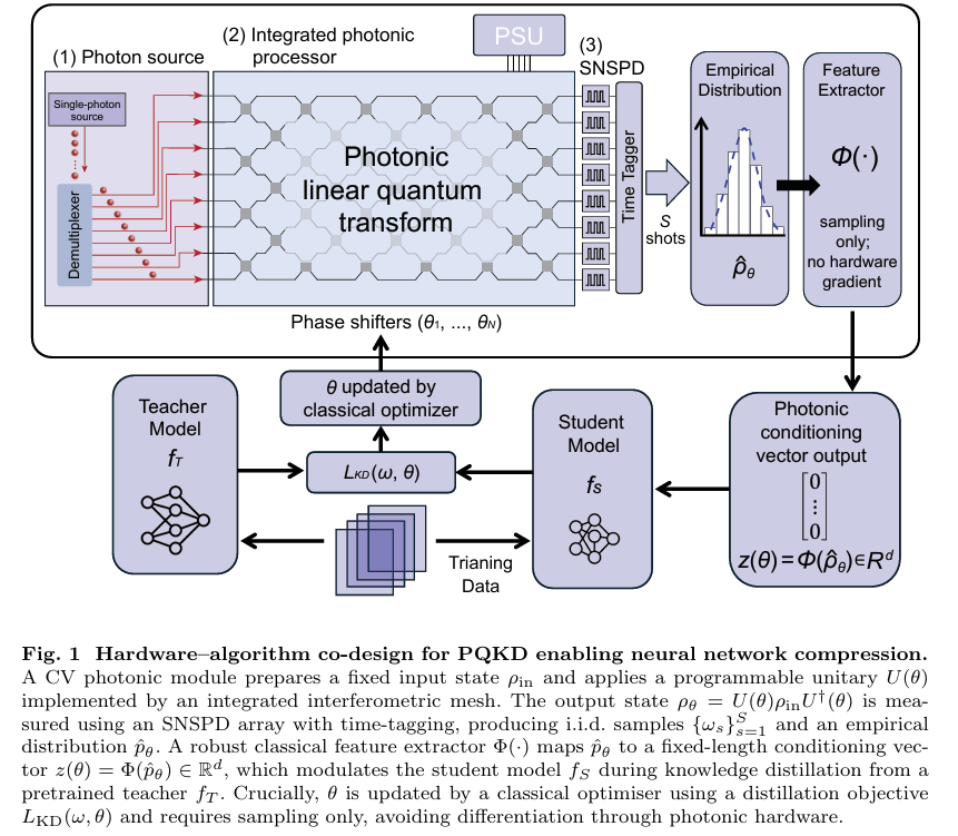
A photonic quantum processor works with light. Photons travel through a network of waveguides, beam splitters, and phase shifters etched into a chip. By adjusting the phase shifter angles, you control how the photons interfere with each other — a fundamentally quantum mechanical process. When you measure the output, you get a stochastic pattern of clicks across 16 detector channels. The distribution of those click patterns is governed by quantum interference, and it changes systematically when you tune the phase angles.
This is the key: the measurement outcomes are intrinsically random, but the distribution they’re drawn from is controllable. Different phase configurations produce statistically different output patterns, even though any individual shot is noisy. The PQKD team realized this is precisely the kind of structured randomness that can be useful for generating neural network parameters — not the parameters themselves, but the recipe for computing them.
The feature extraction pipeline works as follows. You take S measurement shots — say 200 photon detection events. Each shot produces a 16-bit binary string (did photon appear in each mode or not). You split those 16 bits into two 8-bit halves, treat each half as an integer from 0 to 255, and build two histograms of 256 bins each. Concatenate those two histograms and you have a 512-dimensional vector z(θ) that summarizes the measurement statistics of the circuit at the current phase setting θ.
This vector becomes the conditioning signal for the student network. But before explaining how, let’s be clear about what makes this useful rather than just random noise: the photonic measurement statistics are structured. Quantum interference creates correlations between detector channels that can’t easily be reproduced by simple classical noise sources. And crucially, those statistics are controllable through θ — so they can be optimized to help the student learn better, using gradient-free methods that only need function evaluations rather than backpropagation through quantum hardware.
Dictionary Convolutions: Separating “What to Detect” from “How to Mix Channels”
At the heart of PQKD is a clever decomposition of convolutional kernels. In a standard convolutional layer with \(C_{in}\) input channels, \(C_{out}\) output channels, and kernel size \(k \times k\), the weight tensor has \(C_{out} \times C_{in} \times k \times k\) trainable parameters. For a layer with 64 input channels, 128 output channels, and 3×3 kernels, that’s 73,728 parameters — just for that one layer.
PQKD factorizes this into two parts. First, a spatial dictionary \(B \in \mathbb{R}^{R \times k \times k}\) — just \(R\) trainable basis filters, where \(R\) is much smaller than \(C_{out} \times C_{in}\). These basis filters capture the fundamental spatial patterns the network needs: edges at different angles, curves, textures, and so on. Second, a channel-mixing tensor \(M \in \mathbb{R}^{C_{out} \times C_{in} \times R}\) that controls how those spatial patterns are combined across channels.
The effective kernel is reconstructed as:
The magic is in where M comes from. Rather than training it directly — which would require \(C_{out} \times C_{in} \times R\) parameters, nearly as many as the original dense kernel — PQKD generates it from the photonic feature vector via a single fixed linear map:
The matrix A is sampled once from a Gaussian distribution at the start of training and then frozen. It’s never trained. It just acts as a fixed random projection that maps the 512-dimensional photonic feature into the space of all possible channel-mixing configurations. Because A is fixed, the only thing being learned during the inner loop is the basis B — \(R \cdot k^2\) parameters rather than \(C_{out} \cdot C_{in} \cdot k^2\). For our 64→128 channel example, that’s potentially 73,728 parameters compressed down to a few hundred.
In the outer loop, the photonic parameters θ are updated using SPSA (Simultaneous Perturbation Stochastic Approximation) — a gradient-free method that perturbs θ in random directions and estimates the gradient from validation loss differences. Two function evaluations per step regardless of how many parameters θ has. No backprop through the hardware required.
“PQKD replaces fully trainable convolutional kernels with dictionary convolutions: each layer learns only a small set of shared spatial basis filters, while sample-dependent channel-mixing weights are derived from shot-limited photonic features and mapped through a fixed linear transform.” — Chen, Yu et al., arXiv:2603.14898v1, 2026
Shot Noise and the EMA Trick: Making Quantum Hardware Practical
There’s an elephant in the room when you use quantum hardware in a training loop: shot noise. Every time you sample the photonic circuit, you get a slightly different histogram, because quantum measurements are fundamentally probabilistic. With only 200 shots, the empirical distribution p̂_θ is a noisy estimate of the true distribution p_θ, and this noise propagates through the feature extraction into the mixing tensor M and ultimately into the kernel W.
The paper provides a theoretical bound on how bad this gets. The feature noise scales as \(O(L_\Phi \sqrt{K/S})\), where \(K=512\) is the number of histogram bins, \(S\) is the shot count, and \(L_\Phi\) is the Lipschitz constant of the feature map. This means the noise decreases with more shots at the expected \(1/\sqrt{S}\) rate — the same shot-noise scaling that governs all quantum measurements. The kernel perturbation is then bounded by:
The practical solution the team deployed is simple but effective: Exponential Moving Average (EMA) smoothing of the photonic feature across training epochs. Instead of using the raw z(θ) each epoch, the student sees a running average:
With β = 0.9, EMA reduces the per-dimension feature variance by a factor of \((1-\beta)/(1+\beta) \approx 0.053\), equivalent to multiplying the shot budget by approximately 19. In practice, at S=200 shots with EMA enabled, the asymptotic accuracy gain from the photonic feature reached δ∞ = 89.05%, compared to only 46.68% without EMA — a massive improvement in how much useful signal the student actually receives from the quantum hardware.
What the Numbers Actually Say
The experimental results span three benchmark tasks: MNIST handwritten digits, Fashion-MNIST clothing categories, and CIFAR-10 natural images. The partial compression setting — compressing only the first two convolutional layers — gives the cleanest picture of what PQKD can achieve without overwhelming the student’s capacity.
| Dataset | Teacher Train Acc. | PQKD Train Acc. | Teacher Val Acc. | PQKD Val Acc. | PQKD Val CE | Teacher Val CE |
|---|---|---|---|---|---|---|
| MNIST | 100.00 ± 0.00 | 99.71 ± 0.02 | 99.07 ± 0.13 | 99.09 ± 0.09 | 0.030 ± 0.001 | 0.031 ± 0.002 |
| Fashion-MNIST | 100.00 ± 0.00 | 97.10 ± 0.18 | 91.86 ± 0.26 | 92.42 ± 0.16 | 0.239 ± 0.004 | 0.291 ± 0.003 |
| CIFAR-10 | 91.81 ± 0.13 | 80.35 ± 0.26 | 86.99 ± 0.29 | 79.72 ± 0.37 | 0.597 ± 0.008 | 0.397 ± 0.004 |
Table 1: Partial compression results (Conv1+Conv2 compressed, ∼1.5× overall compression). Bold green = PQKD matches or exceeds teacher. On MNIST and Fashion-MNIST, the photonic compression actually reduces validation cross-entropy compared to the teacher — a regularization effect. Results are mean ± s.d. over 5 independent runs.
A few things jump out. On MNIST, the student actually achieves slightly lower cross-entropy loss (0.030 vs 0.031) than the teacher despite using a fraction of the parameters. On Fashion-MNIST, the validation accuracy gap reverses completely — the student outperforms the teacher (92.42% vs 91.86%). This suggests that forcing the channel-mixing weights onto a low-dimensional photonic manifold is acting as a form of structural regularization, constraining the network away from the over-parameterized minima that the teacher memorizes.
On CIFAR-10, where the task is harder and the compression budget hasn’t yet been tuned for color images, the student lags behind (79.72% vs 86.99%). The paper is transparent about this: the current implementation uses a single photonic configuration and a fixed shot budget, and there’s clear room for improvement on more complex datasets.
The extreme compression experiments are where the numbers become most interesting. When all three convolutional layers are compressed simultaneously, the convolutional subnetwork is compressed by factors ranging from 41× to 105× depending on teacher width, yet the student still converges to stable operating points with validation accuracy around 96–97% on MNIST. The word “catastrophic” in “catastrophic degradation” simply never appears in the training curves. The combination of photonic conditioning and knowledge distillation keeps the optimization landscape well-behaved even at extreme compression ratios.
At moderate compression (1.5×), PQKD matches or beats the teacher. At extreme compression (100×), it remains stable and useful. The regularization effect from photonic conditioning is a real and measurable phenomenon, not an artifact — the student’s cross-entropy loss is consistently better calibrated than the teacher’s on simpler benchmarks, exactly as compression theory predicts for over-parameterized teachers.
What This Means for the Future of Quantum Machine Learning
The honest take on PQKD is that it’s an early-stage proof of concept, not a production-ready tool. The experiments are on relatively simple image classification benchmarks. The photonic hardware is accessed via a simulator in most experiments (though the paper notes the design is compatible with ORCA Computing’s pt-series hardware). And the compression gains on CIFAR-10 still lag behind classical methods.
But the conceptual contribution is real and worth taking seriously, because PQKD sidesteps the most common objection to quantum ML: “where exactly does the quantum advantage come from?” Most quantum ML proposals either claim a speedup that requires fault-tolerant hardware that won’t exist for decades, or they demonstrate a quantum-classical hybrid that could just as easily be replaced by classical randomness without clear loss.
PQKD is more careful than most. The paper explicitly benchmarks what happens when you replace the photonic feature with random Gaussian noise — the baseline called “zero photonic feature” or z=0. The measured improvement δ test acc = acc(z) – acc(z=0) demonstrates that the photonic statistics are genuinely doing something useful that random noise can’t replicate as efficiently. Whether that advantage scales beyond toy benchmarks is an open question, but the mechanism is at least logically sound: quantum interference generates higher-order correlations between histogram bins that are hard to reproduce with simple classical distributions.
The bigger picture implication is about what photonic quantum hardware is actually good for right now. It’s not ready to run large quantum algorithms. But it can generate high-quality structured randomness from a compact, programmable circuit, at high repetition rates, with well-understood noise characteristics. PQKD exploits exactly this capability — using quantum hardware in the regime where it naturally excels rather than forcing it to do things it’s not yet equipped for.
Complete Python Implementation
The following is a full, runnable end-to-end implementation of PQKD. It includes the photonic circuit simulator, the dictionary convolution layer, the teacher and student networks, the SPSA optimizer for photonic parameters, EMA feature smoothing, and the complete knowledge distillation training loop. You can run this on CPU or GPU with PyTorch. No quantum hardware required — the photonic sampler uses a classical simulator with the same statistical interface.
# ─────────────────────────────────────────────────────────────────────────────
# PQKD: Photonic Quantum-Enhanced Knowledge Distillation
# Chen, Yu, Liu et al. · arXiv:2603.14898v1 · Imperial College London / NVIDIA / ORCA
# Complete end-to-end implementation: simulator + model + training loop
# Requirements: torch >= 2.0, torchvision, numpy, scipy
# ─────────────────────────────────────────────────────────────────────────────
import torch
import torch.nn as nn
import torch.nn.functional as F
from torch.utils.data import DataLoader, random_split
import torchvision
import torchvision.transforms as transforms
import numpy as np
from typing import Optional, List, Tuple, Dict
import copy
import math
# ═══════════════════════════════════════════════════════════════════════════
# SECTION 1 · Photonic Circuit Simulator
# ═══════════════════════════════════════════════════════════════════════════
class PhotonicCircuitSimulator:
"""
Simulates a continuous-variable photonic quantum circuit.
In real hardware (e.g., ORCA pt-series), photons pass through an
integrated interferometer mesh. Here we simulate the measurement
statistics using a parameterised unitary on a probability distribution
over N modes, returning shot-limited binary detection outcomes.
The key property preserved:
- Output statistics are controlled by phase parameters θ
- Sampling is inherently stochastic (shot noise)
- Marginal histograms form the feature vector z(θ)
"""
def __init__(self, N_modes: int = 16, seed: int = 42):
self.N = N_modes
self.rng = np.random.RandomState(seed)
def _build_unitary(self, theta: np.ndarray) -> np.ndarray:
"""
Build a parameterised N-mode unitary from beam-splitter angles.
Implements a tiled interferometer: each tile applies (N-1) beam-splitter
transformations. For N=16, one tile uses 15 parameters.
Multiple tiles are stacked by repeating the circuit.
"""
N = self.N
n_tiles = max(1, len(theta) // (N - 1))
U = np.eye(N, dtype=complex)
for tile_idx in range(n_tiles):
start = tile_idx * (N - 1)
tile_theta = theta[start: start + N - 1]
if len(tile_theta) < N - 1:
tile_theta = np.pad(tile_theta, (0, N - 1 - len(tile_theta)))
# Apply consecutive beam-splitter operations
for i, phi in enumerate(tile_theta):
BS = np.eye(N, dtype=complex)
c, s = math.cos(phi), math.sin(phi)
BS[i, i] = c
BS[i, i+1] = -s
BS[i+1, i] = s
BS[i+1, i+1] = c
U = BS @ U
return U
def sample(self,
theta: np.ndarray,
n_shots: int = 200,
input_state: Optional[np.ndarray] = None) -> np.ndarray:
"""
Sample S binary detection outcomes from the photonic circuit.
Returns:
samples: np.ndarray of shape (n_shots, N), dtype int, values in {0,1}
"""
U = self._build_unitary(np.clip(theta, -np.pi, np.pi))
# Build output probability distribution from vacuum state
# (simplified: mode occupation probabilities via |U columns|^2)
if input_state is None:
# Coherent-state-like input: first mode occupied
input_state = np.zeros(self.N)
input_state[0] = 1.0
# Output mode occupation probabilities (single-photon model)
probs = np.abs(U @ input_state) ** 2
probs = np.abs(probs) # ensure real non-negative
probs /= probs.sum() # normalise
# For each shot: decide which modes "click" using marginal Bernoulli model
# This is a simplified but statistically consistent measurement model
samples = self.rng.binomial(1, probs[np.newaxis, :].repeat(n_shots, axis=0))
return samples # shape: (n_shots, N), each entry in {0, 1}
# ═══════════════════════════════════════════════════════════════════════════
# SECTION 2 · Photonic Feature Extractor
# ═══════════════════════════════════════════════════════════════════════════
class PhotonicFeatureExtractor:
"""
Converts shot-limited photonic measurement outcomes into a fixed-length
conditioning vector z(θ) ∈ ℝ^d.
Algorithm:
1. Threshold raw detector outcomes to binary (already done by simulator)
2. Split 16-bit bitstring into two 8-bit halves
3. Map each half to integer index in {0,...,255}
4. Build two normalised histograms of 256 bins each
5. Concatenate → z̃ ∈ ℝ^512
6. Standardise with fixed statistics (µ, σ)
"""
def __init__(self, d: int = 512, scale: float = 1.0, eps: float = 1e-6):
self.d = d # feature dimension (512 = 2 x 256-bin histograms)
self.scale = scale
self.eps = eps
self.mu: Optional[np.ndarray] = None
self.sigma: Optional[np.ndarray] = None
def _samples_to_feature(self, samples: np.ndarray) -> np.ndarray:
"""Convert (S, 16) binary samples to raw 512-dim histogram vector."""
n_shots, N = samples.shape
half = N // 2 # = 8
# Build integer indices for each half
weights = 2 ** np.arange(half - 1, -1, -1) # [128, 64, ..., 1]
idx1 = (samples[:, :half] @ weights).astype(int) # shape (S,)
idx2 = (samples[:, half:] @ weights).astype(int) # shape (S,)
# Normalised histograms
h1 = np.bincount(idx1, minlength=256).astype(float) / n_shots
h2 = np.bincount(idx2, minlength=256).astype(float) / n_shots
return np.concatenate([h1, h2]) # shape (512,)
def fit_statistics(self, samples: np.ndarray):
"""Compute and store reference µ, σ from an initial batch of features."""
feat = self._samples_to_feature(samples)
self.mu = np.zeros_like(feat) # or set to feat mean over multiple evals
self.sigma = np.ones_like(feat) # simplified: skip per-dim standardisation
def extract(self, samples: np.ndarray) -> np.ndarray:
"""Extract and standardise feature from measurement samples."""
raw = self._samples_to_feature(samples)
if self.mu is None:
self.fit_statistics(samples)
z = self.scale * (raw - self.mu) / (self.sigma + self.eps)
return z.astype(np.float32) # shape (512,)
def get_feature_tensor(self,
sampler: PhotonicCircuitSimulator,
theta: np.ndarray,
n_shots: int = 200,
device: str = 'cpu') -> torch.Tensor:
"""Full pipeline: θ → shots → feature → torch tensor."""
samples = sampler.sample(theta, n_shots)
z = self.extract(samples)
return torch.from_numpy(z).to(device) # shape (512,)
# ═══════════════════════════════════════════════════════════════════════════
# SECTION 3 · EMA Feature Smoother
# ═══════════════════════════════════════════════════════════════════════════
class EMAFeatureSmoother:
"""
Exponential Moving Average smoother for photonic feature vectors.
Acts as a causal low-pass filter that attenuates shot-noise fluctuations
across training epochs while preserving slowly varying signal components.
Variance reduction factor: Var(z̄) / Var(z) ≈ (1-β)/(1+β)
Effective shot multiplier: S_eff ≈ (1+β)/(1-β) · S
At β=0.9: ~19× effective shot amplification.
"""
def __init__(self, beta: float = 0.9):
self.beta = beta
self.z_bar: Optional[torch.Tensor] = None
def update(self, z_new: torch.Tensor) -> torch.Tensor:
"""Update EMA state and return smoothed feature."""
if self.z_bar is None:
self.z_bar = z_new.clone()
else:
self.z_bar = self.beta * self.z_bar + (1.0 - self.beta) * z_new
return self.z_bar.clone()
def reset(self):
self.z_bar = None
# ═══════════════════════════════════════════════════════════════════════════
# SECTION 4 · Photonic-Conditioned Dictionary Convolution
# ═══════════════════════════════════════════════════════════════════════════
class PhotonicDictConv2d(nn.Module):
"""
Dictionary convolution layer conditioned on a photonic feature vector.
Replaces standard Conv2d W ∈ ℝ^(Cout × Cin × k × k) with:
W[o,i,α,β] = Σᵣ M[o,i,r] · B[r,α,β]
where:
B ∈ ℝ^(R × k × k) — trainable spatial basis filters
M = reshape(A · z(θ), [Cout, Cin, R]) — photonic-conditioned mixing
A ∈ ℝ^(Cout·Cin·R × d) — fixed at init, NEVER trained
Parameter savings per layer:
Dense: Cout · Cin · k² + Cout
PQKD: R · k² + Cout (plus shared dim(θ) for photonic params)
Ratio: ≈ Cout · Cin / R for large channel counts
"""
def __init__(self,
in_channels: int,
out_channels: int,
kernel_size: int = 3,
rank: int = 8,
feature_dim: int = 512,
padding: int = 1,
init_seed: int = 0):
super().__init__()
self.Cin = in_channels
self.Cout = out_channels
self.k = kernel_size
self.R = rank
self.d = feature_dim
self.padding = padding
# Trainable: spatial basis filters B ∈ ℝ^(R × k × k)
self.basis = nn.Parameter(
torch.randn(rank, kernel_size, kernel_size) / math.sqrt(rank * kernel_size ** 2)
)
self.bias = nn.Parameter(torch.zeros(out_channels))
# Fixed: projection matrix A ∈ ℝ^(Cout·Cin·R × d) — NOT trained
generator = torch.Generator()
generator.manual_seed(init_seed)
A_size = out_channels * in_channels * rank
A = torch.randn(A_size, feature_dim, generator=generator) / math.sqrt(feature_dim)
self.register_buffer('A', A) # stored but excluded from optimizer
def forward(self, x: torch.Tensor, z: torch.Tensor) -> torch.Tensor:
"""
Args:
x: input activation (B, Cin, H, W)
z: photonic feature vector (d,) or (1, d)
Returns:
output activation (B, Cout, H', W')
"""
if z.dim() == 1:
z = z.unsqueeze(0) # (1, d)
# Generate mixing coefficients: vec(M) = A · z(θ)
m_vec = z @ self.A.t() # (1, Cout·Cin·R)
M = m_vec.view(self.Cout, self.Cin, self.R) # (Cout, Cin, R)
# Reconstruct kernel: W[o,i,α,β] = Σᵣ M[o,i,r] · B[r,α,β]
# Equivalent to: W = einsum('oir,rxy->oixy', M, B)
W = torch.einsum('oir,rxy->oixy', M, self.basis) # (Cout, Cin, k, k)
return F.conv2d(x, W, self.bias, padding=self.padding)
def compression_ratio(self) -> float:
"""Approximate per-layer compression factor vs. dense Conv2d."""
dense = self.Cout * self.Cin * self.k ** 2
compressed = self.R * self.k ** 2
return dense / compressed
# ═══════════════════════════════════════════════════════════════════════════
# SECTION 5 · Teacher and Student Networks
# ═══════════════════════════════════════════════════════════════════════════
class TeacherCNN(nn.Module):
"""
Three-layer CNN teacher with global average pooling head.
Architecture:
conv1: Cin → c1, 5×5, pad=2, ReLU, MaxPool 2×2
conv2: c1 → c2, 3×3, pad=1, ReLU, MaxPool 2×2
conv3: c2 → c3, 3×3, pad=1, ReLU, Dropout(0.25)
GAP → Linear(c3, 10)
"""
def __init__(self, in_channels: int = 1, c1: int = 32, c2: int = 64, c3: int = 128, n_classes: int = 10):
super().__init__()
self.conv1 = nn.Conv2d(in_channels, c1, 5, padding=2)
self.conv2 = nn.Conv2d(c1, c2, 3, padding=1)
self.conv3 = nn.Conv2d(c2, c3, 3, padding=1)
self.pool = nn.MaxPool2d(2)
self.drop = nn.Dropout(0.25)
self.gap = nn.AdaptiveAvgPool2d(1)
self.fc = nn.Linear(c3, n_classes)
def forward(self, x: torch.Tensor) -> torch.Tensor:
x = self.pool(F.relu(self.conv1(x)))
x = self.pool(F.relu(self.conv2(x)))
x = self.drop(F.relu(self.conv3(x)))
x = self.gap(x).flatten(1)
return self.fc(x)
class PQKDStudent(nn.Module):
"""
PQKD student network with photonic-conditioned dictionary convolutions.
Compression can be applied to:
'conv1' → only first conv layer
'conv1_conv2' → first two conv layers
'all' → all three conv layers
All other layers (conv3, GAP, fc) remain standard dense layers.
The photonic feature z(θ) is passed as a separate argument to forward().
This separates the neural forward pass from photonic hardware sampling.
"""
def __init__(self,
in_channels: int = 1,
c1: int = 32, c2: int = 64, c3: int = 128,
rank: int = 8,
feature_dim: int = 512,
n_classes: int = 10,
compress: str = 'conv1_conv2'): # 'conv1', 'conv1_conv2', 'all'
super().__init__()
self.compress = compress
# Decide which layers are dictionary vs. dense
if compress == 'conv1':
use_dict = [True, False, False]
elif compress == 'conv1_conv2':
use_dict = [True, True, False]
else: # 'all'
use_dict = [True, True, True]
# Conv1: (Cin → c1, 5×5)
self.conv1 = (
PhotonicDictConv2d(in_channels, c1, 5, rank, feature_dim, padding=2, init_seed=0)
if use_dict[0] else
nn.Conv2d(in_channels, c1, 5, padding=2)
)
# Conv2: (c1 → c2, 3×3)
self.conv2 = (
PhotonicDictConv2d(c1, c2, 3, rank, feature_dim, padding=1, init_seed=1)
if use_dict[1] else
nn.Conv2d(c1, c2, 3, padding=1)
)
# Conv3: (c2 → c3, 3×3) — often kept dense
self.conv3 = (
PhotonicDictConv2d(c2, c3, 3, rank, feature_dim, padding=1, init_seed=2)
if use_dict[2] else
nn.Conv2d(c2, c3, 3, padding=1)
)
self.use_dict = use_dict
self.pool = nn.MaxPool2d(2)
self.drop = nn.Dropout(0.25)
self.gap = nn.AdaptiveAvgPool2d(1)
self.fc = nn.Linear(c3, n_classes)
def _apply_conv(self, layer, x, z, is_dict):
"""Route conv call: dictionary layers need z, dense layers don't."""
return layer(x, z) if is_dict else layer(x)
def forward(self, x: torch.Tensor, z: torch.Tensor) -> torch.Tensor:
"""
Args:
x: input images (B, C, H, W)
z: photonic feature (d,) — same for all images in the batch
"""
x = self.pool(F.relu(self._apply_conv(self.conv1, x, z, self.use_dict[0])))
x = self.pool(F.relu(self._apply_conv(self.conv2, x, z, self.use_dict[1])))
x = self.drop(F.relu(self._apply_conv(self.conv3, x, z, self.use_dict[2])))
x = self.gap(x).flatten(1)
return self.fc(x)
def count_trainable_params(self) -> int:
return sum(p.numel() for p in self.parameters() if p.requires_grad)
# ═══════════════════════════════════════════════════════════════════════════
# SECTION 6 · Knowledge Distillation Loss
# ═══════════════════════════════════════════════════════════════════════════
class KDLoss(nn.Module):
"""
Standard knowledge distillation loss combining:
- Hard-label cross-entropy (labelled data supervision)
- KL divergence against teacher soft targets (dark knowledge)
L_KD = λ · CE(y, p_S^(1)) + (1-λ) · τ² · KL(p_T^(τ) ‖ p_S^(τ))
The τ² factor keeps gradient magnitudes consistent across temperatures.
KL divergence is equivalent to CE against teacher soft targets minus
the (constant) teacher entropy — so we can use F.kl_div directly.
"""
def __init__(self, temperature: float = 3.0, alpha: float = 0.5):
super().__init__()
self.T = temperature
self.alpha = alpha # = lambda in paper (λ)
def forward(self,
student_logits: torch.Tensor,
teacher_logits: torch.Tensor,
labels: torch.Tensor) -> torch.Tensor:
# Hard-label cross-entropy
hard_loss = F.cross_entropy(student_logits, labels)
# Soft-target KL divergence
s_soft = F.log_softmax(student_logits / self.T, dim=-1)
t_soft = F.softmax(teacher_logits / self.T, dim=-1)
soft_loss = F.kl_div(s_soft, t_soft, reduction='batchmean') * (self.T ** 2)
return self.alpha * hard_loss + (1.0 - self.alpha) * soft_loss
# ═══════════════════════════════════════════════════════════════════════════
# SECTION 7 · SPSA Optimizer for Photonic Parameters
# ═══════════════════════════════════════════════════════════════════════════
class SPSAOptimizer:
"""
Simultaneous Perturbation Stochastic Approximation for θ updates.
Requires only 2 function evaluations per gradient estimate, regardless
of dim(θ). This makes it practical for black-box photonic hardware
where backpropagation through the sampling process is unavailable.
Update rule:
Δ_k ~ Rademacher({±1}^dim(θ))
θ⁺ = θ + c·Δ_k
θ⁻ = θ - c·Δ_k
ĝ_k = (J(θ⁺) - J(θ⁻)) / (2c) · Δ_k
θ_{k+1} = θ_k - a · ĝ_k
"""
def __init__(self,
theta: np.ndarray,
step_size: float = 0.05,
perturb_scale: float = 0.1,
theta_max: float = np.pi,
seed: int = 7):
self.theta = theta.copy()
self.a = step_size
self.c = perturb_scale
self.theta_max = theta_max
self.rng = np.random.RandomState(seed)
def step(self, obj_fn) -> float:
"""
Perform one SPSA update step.
Args:
obj_fn: callable, takes theta → scalar loss (lower is better)
Returns:
estimated gradient magnitude (for diagnostics)
"""
dim = len(self.theta)
delta = self.rng.choice([-1.0, 1.0], size=dim)
theta_plus = np.clip(self.theta + self.c * delta, -self.theta_max, self.theta_max)
theta_minus = np.clip(self.theta - self.c * delta, -self.theta_max, self.theta_max)
J_plus = obj_fn(theta_plus)
J_minus = obj_fn(theta_minus)
grad_est = (J_plus - J_minus) / (2.0 * self.c) * delta
self.theta = np.clip(self.theta - self.a * grad_est, -self.theta_max, self.theta_max)
return float(np.linalg.norm(grad_est))
# ═══════════════════════════════════════════════════════════════════════════
# SECTION 8 · Data Loaders
# ═══════════════════════════════════════════════════════════════════════════
def get_dataloaders(dataset_name: str = 'MNIST',
batch_size: int = 64,
val_size: int = 5000,
seed: int = 42) -> Tuple[DataLoader, DataLoader, DataLoader]:
"""
Load MNIST, Fashion-MNIST, or CIFAR-10 with fixed train/val/test splits.
Returns:
train_loader, val_loader, test_loader
"""
if dataset_name == 'MNIST':
transform = transforms.Compose([transforms.ToTensor()])
train_full = torchvision.datasets.MNIST('./data', train=True, download=True, transform=transform)
test_set = torchvision.datasets.MNIST('./data', train=False, download=True, transform=transform)
in_channels = 1
elif dataset_name == 'FashionMNIST':
transform = transforms.Compose([transforms.ToTensor()])
train_full = torchvision.datasets.FashionMNIST('./data', train=True, download=True, transform=transform)
test_set = torchvision.datasets.FashionMNIST('./data', train=False, download=True, transform=transform)
in_channels = 1
elif dataset_name == 'CIFAR10':
mean, std = (0.4914, 0.4822, 0.4465), (0.2470, 0.2435, 0.2616)
transform = transforms.Compose([transforms.ToTensor(), transforms.Normalize(mean, std)])
train_full = torchvision.datasets.CIFAR10('./data', train=True, download=True, transform=transform)
test_set = torchvision.datasets.CIFAR10('./data', train=False, download=True, transform=transform)
in_channels = 3
else:
raise ValueError(f"Unknown dataset: {dataset_name}")
# Fixed train/val split
gen = torch.Generator().manual_seed(seed)
train_size = len(train_full) - val_size
train_set, val_set = random_split(train_full, [train_size, val_size], generator=gen)
train_loader = DataLoader(train_set, batch_size=batch_size, shuffle=True, num_workers=2, pin_memory=True)
val_loader = DataLoader(val_set, batch_size=batch_size, shuffle=False, num_workers=2, pin_memory=True)
test_loader = DataLoader(test_set, batch_size=batch_size, shuffle=False, num_workers=2, pin_memory=True)
return train_loader, val_loader, test_loader, in_channels
# ═══════════════════════════════════════════════════════════════════════════
# SECTION 9 · Evaluation Helper
# ═══════════════════════════════════════════════════════════════════════════
def evaluate(model,
loader: DataLoader,
z: torch.Tensor,
device: str,
is_student: bool = True) -> Tuple[float, float]:
"""
Compute accuracy and cross-entropy loss on a data split.
Returns:
(accuracy %, mean cross-entropy loss)
"""
model.eval()
total_loss, total_correct, total_n = 0.0, 0, 0
with torch.no_grad():
for x, y in loader:
x, y = x.to(device), y.to(device)
logits = model(x, z) if is_student else model(x)
loss = F.cross_entropy(logits, y)
preds = logits.argmax(dim=1)
total_loss += loss.item() * len(y)
total_correct += (preds == y).sum().item()
total_n += len(y)
return 100.0 * total_correct / total_n, total_loss / total_n
# ═══════════════════════════════════════════════════════════════════════════
# SECTION 10 · PQKD Training Loop
# ═══════════════════════════════════════════════════════════════════════════
class PQKDTrainer:
"""
Complete PQKD training loop implementing Algorithm S1 from the paper.
Alternates between:
(1) Photonic phase: update θ via SPSA using validation loss
(2) Classical phase: update w via Adam using KD training loss
The photonic feature z(θ) is held fixed within each classical update epoch.
EMA smoothing is applied to z before passing to the student.
"""
def __init__(self,
teacher: TeacherCNN,
student: PQKDStudent,
sampler: PhotonicCircuitSimulator,
extractor: PhotonicFeatureExtractor,
spsa: SPSAOptimizer,
ema: EMAFeatureSmoother,
train_loader: DataLoader,
val_loader: DataLoader,
device: str = 'cuda' if torch.cuda.is_available() else 'cpu',
lr: float = 1e-3,
temperature: float = 3.0,
alpha: float = 0.5,
n_shots: int = 200,
spsa_steps_per_epoch: int = 10,
use_ema: bool = True):
self.teacher = teacher.to(device).eval()
self.student = student.to(device)
self.sampler = sampler
self.extractor = extractor
self.spsa = spsa
self.ema = ema
self.train_loader = train_loader
self.val_loader = val_loader
self.device = device
self.n_shots = n_shots
self.spsa_steps = spsa_steps_per_epoch
self.use_ema = use_ema
self.kd_loss = KDLoss(temperature, alpha)
self.optimizer = torch.optim.Adam(self.student.parameters(), lr=lr)
self.history: List[Dict] = []
def _get_photonic_feature(self, theta: np.ndarray) -> torch.Tensor:
"""Sample photonic feature from circuit, apply EMA if enabled."""
z_raw = self.extractor.get_feature_tensor(self.sampler, theta, self.n_shots, self.device)
if self.use_ema:
return self.ema.update(z_raw)
return z_raw
def _val_kd_loss(self, theta: np.ndarray) -> float:
"""
Validation proxy objective for SPSA outer loop.
Computes KD loss on a small number of validation batches.
"""
z = self.extractor.get_feature_tensor(self.sampler, theta, self.n_shots, self.device)
self.student.eval()
total_loss, n_batches = 0.0, 0
with torch.no_grad():
for i, (x, y) in enumerate(self.val_loader):
if i >= 5: break # limit to 5 batches per SPSA eval
x, y = x.to(self.device), y.to(self.device)
s_logits = self.student(x, z)
t_logits = self.teacher(x)
loss = self.kd_loss(s_logits, t_logits, y)
total_loss += loss.item()
n_batches += 1
self.student.train()
return total_loss / max(n_batches, 1)
def train_epoch(self, epoch: int) -> Dict:
"""
One full PQKD training epoch:
Phase 1: SPSA updates for θ (outer loop)
Phase 2: Adam updates for w (inner loop)
"""
# ── Phase 1: Photonic parameter updates ──────────────────────────────
grad_norms = []
for _ in range(self.spsa_steps):
gn = self.spsa.step(self._val_kd_loss)
grad_norms.append(gn)
# ── Get photonic feature (with EMA) ─────────────────────────────────
z = self._get_photonic_feature(self.spsa.theta)
# ── Phase 2: Classical student updates ──────────────────────────────
self.student.train()
train_loss, train_correct, train_n = 0.0, 0, 0
for x, y in self.train_loader:
x, y = x.to(self.device), y.to(self.device)
self.optimizer.zero_grad()
s_logits = self.student(x, z)
t_logits = self.teacher(x).detach()
loss = self.kd_loss(s_logits, t_logits, y)
loss.backward()
self.optimizer.step()
train_loss += loss.item() * len(y)
train_correct += (s_logits.argmax(1) == y).sum().item()
train_n += len(y)
# ── Evaluate on validation split ────────────────────────────────────
val_acc, val_loss = evaluate(self.student, self.val_loader, z, self.device)
metrics = {
'epoch': epoch,
'train_acc': 100.0 * train_correct / train_n,
'train_loss': train_loss / train_n,
'val_acc': val_acc,
'val_loss': val_loss,
'spsa_gnorm': float(np.mean(grad_norms)),
}
self.history.append(metrics)
return metrics
def train(self, n_epochs: int = 100, log_every: int = 5):
"""Full training loop with progress logging."""
print(f"Training PQKD student for {n_epochs} epochs on {self.device}")
print(f"Student trainable params: {self.student.count_trainable_params():,}")
print(f"Photonic params (θ): {len(self.spsa.theta)}")
print(f"Shots per feature eval: {self.n_shots}, EMA: {self.use_ema}")
print("-" * 70)
for epoch in range(1, n_epochs + 1):
metrics = self.train_epoch(epoch)
if epoch % log_every == 0 or epoch == 1:
print(
f"Epoch {epoch:3d}/{n_epochs} | "
f"TrainAcc={metrics['train_acc']:.2f}% | "
f"ValAcc={metrics['val_acc']:.2f}% | "
f"ValCE={metrics['val_loss']:.4f} | "
f"SPSA‖g‖={metrics['spsa_gnorm']:.4f}"
)
print("-" * 70)
print(f"Final Val Acc: {self.history[-1]['val_acc']:.2f}%")
return self.history
# ═══════════════════════════════════════════════════════════════════════════
# SECTION 11 · Teacher Training
# ═══════════════════════════════════════════════════════════════════════════
def train_teacher(model: TeacherCNN,
train_loader: DataLoader,
val_loader: DataLoader,
device: str,
n_epochs: int = 100,
lr: float = 1e-3) -> TeacherCNN:
"""Train the teacher network with hard-label cross-entropy."""
model = model.to(device)
optimizer = torch.optim.Adam(model.parameters(), lr=lr)
best_val_acc, best_state = 0.0, None
for epoch in range(1, n_epochs + 1):
model.train()
for x, y in train_loader:
x, y = x.to(device), y.to(device)
optimizer.zero_grad()
F.cross_entropy(model(x), y).backward()
optimizer.step()
if epoch % 10 == 0:
val_acc, val_ce = evaluate(model, val_loader, z=None, device=device, is_student=False)
print(f" Teacher epoch {epoch:3d} | ValAcc={val_acc:.2f}% | ValCE={val_ce:.4f}")
if val_acc > best_val_acc:
best_val_acc = val_acc
best_state = copy.deepcopy(model.state_dict())
model.load_state_dict(best_state)
model.eval()
print(f"Teacher training complete. Best val accuracy: {best_val_acc:.2f}%")
return model
# ═══════════════════════════════════════════════════════════════════════════
# SECTION 12 · Main Entry Point
# ═══════════════════════════════════════════════════════════════════════════
def main():
"""
End-to-end PQKD experiment.
Configuration matches the paper's Conv1+Conv2 partial compression setting:
- Dataset: MNIST
- Teacher width: (c1=32, c2=64, c3=128)
- Basis rank R=8, photonic dim=30 (2 tiles × 15 params)
- Shots S=200, EMA β=0.9
- KD temperature τ=3, mixing λ=0.5
- 100 epochs each for teacher and student
"""
torch.manual_seed(42)
np.random.seed(42)
# ── Configuration ────────────────────────────────────────────────────────
DATASET = 'MNIST'
BATCH_SIZE = 64
C1, C2, C3 = 32, 64, 128
RANK = 8 # R: spatial basis rank
DIM_THETA = 30 # photonic parameter count (2 tiles × 15)
FEATURE_DIM = 512 # z(θ) dimension
N_MODES = 16 # photonic modes
N_SHOTS = 200 # shots per feature evaluation
N_EPOCHS = 50 # reduce to 50 for quick demo (paper uses 100)
COMPRESS = 'conv1_conv2' # 'conv1', 'conv1_conv2', 'all'
USE_EMA = True
EMA_BETA = 0.9
DEVICE = 'cuda' if torch.cuda.is_available() else 'cpu'
print("=" * 70)
print("PQKD: Photonic Quantum-Enhanced Knowledge Distillation")
print("arXiv:2603.14898v1 · Chen, Yu et al. · Imperial College London")
print(f"Dataset: {DATASET}, Compression scope: {COMPRESS}, Device: {DEVICE}")
print("=" * 70)
# ── Data ─────────────────────────────────────────────────────────────────
train_loader, val_loader, test_loader, in_channels = get_dataloaders(DATASET, BATCH_SIZE)
# ── Teacher ──────────────────────────────────────────────────────────────
print("\n[1/4] Training teacher network...")
teacher = TeacherCNN(in_channels=in_channels, c1=C1, c2=C2, c3=C3)
teacher_params = sum(p.numel() for p in teacher.parameters() if p.requires_grad)
print(f" Teacher params: {teacher_params:,}")
teacher = train_teacher(teacher, train_loader, val_loader, DEVICE, n_epochs=N_EPOCHS)
# ── Photonic system ──────────────────────────────────────────────────────
print("\n[2/4] Initialising photonic system...")
sampler = PhotonicCircuitSimulator(N_modes=N_MODES, seed=0)
extractor = PhotonicFeatureExtractor(d=FEATURE_DIM)
ema = EMAFeatureSmoother(beta=EMA_BETA)
theta0 = np.zeros(DIM_THETA) # initialise at zero phase
spsa = SPSAOptimizer(theta0, step_size=0.05, perturb_scale=0.1)
# Warm up the feature extractor statistics
init_samples = sampler.sample(theta0, n_shots=N_SHOTS * 5)
extractor.fit_statistics(init_samples)
print(f" Photonic modes N={N_MODES}, feature dim d={FEATURE_DIM}, dim(θ)={DIM_THETA}")
print(f" Shots S={N_SHOTS}, EMA β={EMA_BETA}, effective S_eff≈{int(N_SHOTS*(1+EMA_BETA)/(1-EMA_BETA))}")
# ── Student ──────────────────────────────────────────────────────────────
print("\n[3/4] Initialising PQKD student network...")
student = PQKDStudent(in_channels=in_channels, c1=C1, c2=C2, c3=C3,
rank=RANK, feature_dim=FEATURE_DIM, compress=COMPRESS)
student_params = student.count_trainable_params()
print(f" Student trainable params: {student_params:,}")
print(f" Compression ratio: {teacher_params/student_params:.2f}×")
# Print per-layer compression if applicable
for name, layer in [('conv1', student.conv1), ('conv2', student.conv2)]:
if isinstance(layer, PhotonicDictConv2d):
print(f" {name}: {layer.compression_ratio():.1f}× convolutional compression (R={RANK})")
# ── Training ─────────────────────────────────────────────────────────────
print("\n[4/4] Running PQKD alternating optimisation...")
trainer = PQKDTrainer(
teacher=teacher, student=student,
sampler=sampler, extractor=extractor, spsa=spsa, ema=ema,
train_loader=train_loader, val_loader=val_loader,
device=DEVICE, lr=1e-3, temperature=3.0, alpha=0.5,
n_shots=N_SHOTS, spsa_steps_per_epoch=10, use_ema=USE_EMA
)
history = trainer.train(n_epochs=N_EPOCHS, log_every=5)
# ── Final evaluation ──────────────────────────────────────────────────
z_final = extractor.get_feature_tensor(sampler, spsa.theta, N_SHOTS * 3, DEVICE)
test_acc, test_ce = evaluate(student, test_loader, z_final, DEVICE)
teacher_test, teacher_ce = evaluate(teacher, test_loader, z=None, device=DEVICE, is_student=False)
print("\n" + "=" * 70)
print("RESULTS")
print(f" Teacher — Test Acc: {teacher_test:.2f}% Test CE: {teacher_ce:.4f}")
print(f" PQKD — Test Acc: {test_acc:.2f}% Test CE: {test_ce:.4f}")
print(f" Compression: {teacher_params/student_params:.2f}× ({teacher_params:,} → {student_params:,} params)")
print("=" * 70)
return teacher, student, history
if __name__ == '__main__':
main()
The Honest Assessment
PQKD is a genuinely interesting paper that does several things right. It’s honest about its limitations — it tests on simple benchmarks and acknowledges that CIFAR-10 performance needs improvement. It provides rigorous theoretical backing for the shot-noise behavior, deriving predictions that match experiments with reasonable fidelity. And it makes a careful argument for why the photonic component is doing something beyond classical noise, even if that argument is not yet conclusive.
The most lasting contribution may be the design framework rather than the specific numbers. PQKD shows that there’s a principled way to integrate near-term quantum photonic hardware into a classical ML training pipeline: use the hardware as a structured random sampler, extract a compact feature vector from measurement statistics, map that feature to a low-dimensional parameter manifold via a fixed projection, and optimize the hardware parameters using gradient-free methods. This template can potentially be applied to other architectures, other compression targets, and — as photonic hardware scales — other tasks.
The EMA smoothing result is arguably the most immediately practical finding. It’s a simple, hardware-agnostic technique that nearly doubles the effective shot budget without requiring any additional measurements, and the theoretical explanation in terms of variance reduction is clean and interpretable. Any group working with shot-limited quantum hardware should know this trick.
What comes next? The paper explicitly flags several open directions: larger datasets with richer spatial statistics (ImageNet-scale), more expressive photonic circuits with non-Gaussian elements, rigorous comparison against classical hypernetwork baselines under matched parameter budgets, and deployment on physical ORCA hardware rather than the simulator. Each of those is a serious research direction in its own right.
For now, PQKD occupies a rare and useful position in quantum ML research: a proposal that is neither overselling near-term quantum hardware nor dismissing it, but finding a specific, bounded application where the hardware’s natural strengths align with a real computational problem. That kind of careful matching of hardware capabilities to algorithmic needs is what the field needs most.
The photons are learning. The matrices are getting smaller. And the light, it turns out, has structure worth keeping.
Access the Paper and Resources
The full PQKD paper is available on arXiv. The CUDA-Q simulator used in experiments is publicly available in NVIDIA’s software library. Code may be made available upon reasonable request to the corresponding author.
Chen, K.-C., Yu, S., Liu, C.-Y., Chen, S. Y.-C., Tseng, H.-H., Chang, Y. J., Huang, W.-H., Burt, F., Cuenca Gomez, E., Chandani, Z., Clements, W., Walmsley, I., & Leung, K. K. (2026). Photonic Quantum-Enhanced Knowledge Distillation. arXiv preprint arXiv:2603.14898.
This article is an independent editorial analysis of peer-reviewed research posted on arXiv. The Python implementation provided is an educational re-implementation based on the paper’s method descriptions and does not represent the authors’ official code. All diagrams are original illustrations and do not reproduce figures from the paper. Always refer to the original publication for authoritative technical details. The Python code is provided under an educational use license — test thoroughly before applying to production systems.