How Compressive Sensing Finally Broke the Phase Unwrapping Bottleneck in SAR Interferometry
Researchers at Italy’s CNR-IREA fused decades-old minimum cost flow theory with modern compressive sensing to build a phase unwrapping algorithm that detected a 40 cm volcanic displacement at Stromboli that the classic EMCF method simply could not recover — and did it without requiring any Delaunay triangulation in the temporal domain.
Satellite radar interferometry is one of the most remarkable technologies humans have built: a satellite in orbit emits microwaves, waits for them to bounce back from Earth’s surface, and uses the phase of the returning signal to measure ground movement down to the millimeter scale. The catch is that the phase can only be measured modulo 2π — the satellite essentially gives you only the fractional part of a cycle, never the whole number. Recovering those missing integer multiples (phase unwrapping) is the single most error-prone step in the entire processing chain. For a decade, the Extended Minimum Cost Flow (EMCF) method has been the gold standard for multi-temporal DInSAR analysis. A new paper from CNR-IREA shows that replacing EMCF’s temporal domain solver with a Compressive Sensing L₁-norm minimization — and running multiple spatial unwrapping trials followed by weighted averaging — catches displacement signals that were previously invisible, especially during fast volcanic events.
What Phase Unwrapping Actually Is and Why It Matters
When two SAR images are acquired over the same area at different times, their phase difference forms an interferogram. If the ground moved during that time, the deformation signal appears as fringes in the interferogram — each complete fringe cycle represents roughly half the radar wavelength of movement (about 2.8 cm for Sentinel-1 C-band, ~11 cm for SAOCOM-1 L-band). The problem is that because phase is periodic, the measured interferogram only gives you the fractional part of the total phase within the [−π, +π] interval.
Phase unwrapping recovers the full, continuous deformation signal by figuring out the correct integer number of 2π cycles to add back at each point. This sounds straightforward until you consider: decorrelation noise corrupts some pixels, atmospheric artifacts add spatially correlated phase, residual topography contaminates the signal, and fast volcanic events can create phase gradients large enough that even adjacent coherent pixels differ by more than one full cycle. In those situations, any local-integration approach will accumulate errors that propagate through the entire time series.
The multi-temporal SBAS approach processes not one but hundreds of interferograms simultaneously, which creates both an opportunity and a challenge. The opportunity: temporal consistency across the interferogram stack provides an additional constraint — a pixel that was correctly unwrapped in interferogram 5 should be consistent with interferograms 3 and 8. The challenge: with hundreds of interferograms and potentially millions of coherent pixels, the scale of the problem is enormous, and a PhU error in even one interferogram can propagate into the final deformation time series.
In a multi-temporal interferogram stack, the 2π integer correction vector K is physically sparse — most interferograms in a well-constructed small-baseline stack do not need any correction. Compressive Sensing theory says that sparse vectors can be recovered exactly from underdetermined systems by minimizing the L₁-norm instead of the L₂-norm. This single observation transforms an NP-hard combinatorial problem into a tractable convex optimization, and it liberates the temporal unwrapping step from the Delaunay triangulation constraint that limited EMCF.
The Architecture of the CS-EMCF Algorithm
INPUT: Multi-temporal SAR image stack → wrapped MT-DInSAR interferograms
         │
┌────────▼──────────────────────────────────────────────────────────┐
│  NETWORK GENERATION                                                │
│                                                                    │
│  Temporal network: Delaunay triangulation in TxB⊥ plane           │
│    → select M interferometric pairs from N+1 acquisitions         │
│    → [optional] augment with highly coherent short-baseline pairs │
│                                                                    │
│  Spatial network: Delaunay triangulation in AZxRG plane           │
│    → coherent pixels (triangular coherence γ_tr > 0.90)          │
│    → arcs connecting neighboring coherent pixels                  │
└────────┬──────────────────────────────────────────────────────────┘
         │
┌────────▼──────────────────────────────────────────────────────────┐
│  CS-BASED TEMPORAL PHASE UNWRAPPING  [red dashed box in Fig. 3]  │
│                                                                    │
│  For each arc (AB) in the spatial network:                        │
│                                                                    │
│  Step 1: Linear model estimation                                   │
│    → maximize temporal coherence γ to find (Δz_opt, Δv_opt)      │
│    → compute model m = 4π/λ [Δb⊥/(r·sinθ)·Δz + Δt·Δv]          │
│    → if γ ≥ th_coh: use Φ_hat = m + <Δϕ − m>_2π                 │
│    → else:          use Φ_hat = <Δϕ>_2π                          │
│                                                                    │
│  Step 2: Form under-determined system                             │
│    → Γ·K' = Δϕ_tr   (Q equations, M unknowns, Q << M)           │
│    → Γ is the triangle incidence matrix (network matrix)          │
│                                                                    │
│  Step 3: L1-norm minimization via IRLS                            │
│    → min ‖K'‖₁  s.t. Γ·K' = Δϕ_tr                               │
│    → IRLS weights: w = |(x * b_temp²)^{p_k−2} / 2|               │
│    → iterate until convergence                                    │
│                                                                    │
│  Step 4: Round to nearest integer → K'_rnd                       │
│                                                                    │
│  Step 5: Compute cost function (Eq. 21)                           │
│    → γ_rnd: closeness of K' to K'_rnd (quasi-integer quality)    │
│    → N_corr = ‖K'_rnd‖₀ (sparsity measure)                      │
│    → Cost = 100,000 if (γ_rnd > th_rnd) AND (N_corr < th_sparse) │
│    → Cost = 1 otherwise (arc allowed to vary in spatial PhU)      │
│                                                                    │
│  → Output: unwrapped phase gradients Δψ + cost function array    │
└────────┬──────────────────────────────────────────────────────────┘
         │  (N spatial arcs) × (M interferograms) each with cost
┌────────▼──────────────────────────────────────────────────────────┐
│  MULTI-TRIAL SPATIAL PHASE UNWRAPPING  [blue dashed box]         │
│                                                                    │
│  For T=10 trials, vary thresholds:                                │
│    th_rnd ∈ [0.93, 0.97] (5 values)                              │
│    th_sparse ∈ {5%, 10%}  → 2 sparsity settings                  │
│    → 10 different cost functions total                            │
│                                                                    │
│  For each trial i = 1 … T:                                        │
│    → Run MCF spatial PhU with cost_i                              │
│    → Obtain unwrapped interferogram sequence ψ_i                 │
│    → Run SBAS inversion → time series → synthetic interferograms │
│    → Compute weight w_i = 1 − |<ϕ_i − ϕ_tilde_i>_2π / π|       │
│                                                                    │
│  Weighted average:                                                 │
│    ψ_final = Σ(w_i · ψ_i) / Σ(w_i)   pixel-by-pixel             │
└────────┬──────────────────────────────────────────────────────────┘
         │
OUTPUT: Unwrapped MT-DInSAR interferogram sequence
  → Apply SBAS SVD inversion → LOS deformation time series
  → Validate with temporal coherence Tc (Eq. 24)
Step 1 — Why Delaunay Triangulation Was the Bottleneck
The original EMCF algorithm handles temporal phase unwrapping by building a Delaunay triangulation network in the time/perpendicular-baseline (TxB⊥) plane. Interferograms become the arcs of this network, and triangles in the network represent closed phase loops that must sum to zero — a physical constraint called the irrotational condition. The MCF algorithm then finds the minimum-cost set of integer corrections to enforce this constraint.
The Delaunay triangulation is a sensible choice for dense datasets: it avoids intersecting arcs, guarantees a planar graph, and produces roughly 3× as many interferograms as SAR acquisitions, which is a good redundancy level. But when a SAR dataset has only 22 acquisitions (as in the SAOCOM-1 case study), the resulting triangulation is sparse and weakly constrained. The PhU problem becomes easier to solve incorrectly.
More critically, the MCF algorithm mathematically requires that no two arcs of the network intersect. This means you can never enrich a Delaunay network with additional interferograms that would cross existing arcs — which is exactly what you’d want to do when the network is sparse. The IRLS-based L₁ solver has no such constraint. It solves a linear system of equations, and you can add new equations (corresponding to new interferometric pairs and their triangles) freely, even if their arcs would cross in the TxB⊥ plane.
Step 2 — The L₁-norm Formulation
For a spatial arc connecting pixels A and B, the irrotational condition across all M interferograms can be written as a matrix equation. The network matrix Γ has one row per triangle (Q triangles total) and one column per interferogram (M columns), with entries of +1, −1, or 0 depending on the triangle topology. The phase residual on the right side, Δϕ_tr, captures the closure error that needs to be explained by integer corrections.
Q equations, M unknowns (Q < M), ∞^{M−Q} solutions
Solving this underdetermined system for integer K’ is NP-hard in general (it’s equivalent to sparse signal recovery over integers). But Compressive Sensing theory — specifically the equivalence between sparse L₀-norm minimization and convex L₁-norm minimization under appropriate conditions — converts it to a tractable problem:
The physical justification is direct: in a well-selected small-baseline interferogram stack, the vast majority of arcs between nearby coherent pixels will have phase gradients well within [−π, +π], meaning no integer correction is needed. The correction vector K’ is genuinely sparse. CS can exploit this sparsity to find the unique correct solution even though the system is underdetermined.
Step 3 — The Modified IRLS Solver with Temporal Baseline Weighting
The Iterative Reweighted Least Squares (IRLS) algorithm solves L₁-norm minimization by iteratively solving a sequence of weighted L₂ problems. The key modification from Manunta and Yasir (2022) is introducing the temporal baselines as weights. Longer-baseline interferograms are more likely to have undergone actual deformation, so they carry more uncertainty about whether K’=0. The weight update at each IRLS iteration is:
x = solution at previous iteration, b_temp = temporal baselines vector, p_k = adaptive exponent
An important distinction from prior work: here the IRLS is used to directly implement temporal phase unwrapping, not to correct errors after the fact. The L₁ solution K’ is not constrained to be integer, so a rounding step follows: K’_rnd = round(K’). The quality of this rounding is then quantified by γ_rnd, which measures how close the continuous solution was to an integer — a near-integer solution is a high-confidence unwrapping.
Step 4 — A New Cost Function That Bridges Temporal and Spatial
The original EMCF used the minimum network cost from its temporal MCF solution as a proxy for confidence: low cost means the temporal solver was confident, so the spatial solver should “lock” that arc. The CS-EMCF replaces this with a more physically meaningful cost function:
γ_rnd = quasi-integer quality ∈ [0,1] | N_corr = ‖K’_rnd‖₀ = number of corrected interferograms | Typical: th_rnd = 0.95, th_sparse = 10% of M
An arc with Cost = 100,000 is essentially locked — the spatial MCF algorithm will treat it as a given constraint and build around it. An arc with Cost = 1 is free to be adjusted. The key insight is that this cost function depends jointly on solution quality (γ_rnd) and sparsity (N_corr), so it rewards not just mathematically clean solutions but physically plausible sparse ones.
Step 5 — Multi-Trial Spatial PhU with Weighted Averaging
Any single cost function, no matter how carefully chosen, is an imperfect predictor of which arcs should be locked. Conservative thresholds (high γ_rnd, low N_corr) work well for short arcs between nearby pixels but fail for long arcs spanning areas with large deformation gradients. Permissive thresholds work the other way around. Rather than trying to pick one optimal setting, the algorithm runs T=10 trials with slightly different threshold combinations and combines the results.
For each trial, after the spatial MCF produces an unwrapped interferogram sequence, the algorithm runs a quick SBAS inversion to get the deformation time series, regenerates “synthetic” interferograms from that time series, and computes the phase residuals between measured and synthetic. These residuals directly measure how self-consistent the unwrapped solution is, and they become the weights for the final average:
Weights are per-pixel, per-interferogram — a pixel with excellent residuals in trial i gets high w_i for that trial
The weight w_i ∈ [0,1] where w_i = 1 means perfectly consistent and w_i = 0 means maximally inconsistent. Critically, these weights are computed independently for every pixel in every interferogram — the averaging is not global. A pixel in the active Sciara del Fuoco area might have excellent weights only for the more permissive trial settings (which handle large phase gradients better), while a stable urban pixel might prefer the conservative settings. The algorithm adapts to both simultaneously.
“No single cost function achieves perfect unwrapping — each introduces errors at different interferograms. The weighted average operation significantly reduces the phase residuals in the overall interferometric sequence.” — Yasir, Casu, De Luca et al., ISPRS 2026
Validation Results on Real Volcanic Datasets
SAOCOM-1 at Stromboli — The Small Dataset Case
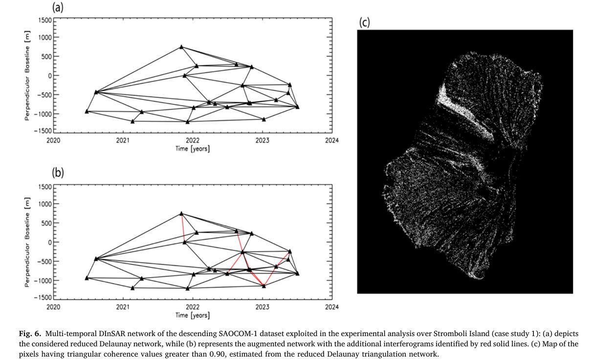
The most demanding test involves only 22 SAOCOM-1 L-band acquisitions over Stromboli Island (June 2020 – July 2023), producing just 54 interferometric pairs through Delaunay triangulation. The Stromboli volcano hosts one of Earth’s most continuously active volcanic systems, with persistent explosive activity and periodic flank movements that can displace the Sciara del Fuoco (the volcano’s lava flow scar) by tens of centimeters.
The reduced Delaunay network struggled to correctly unwrap the Sciara del Fuoco area, failing to recover an April–August 2021 deformation episode. When the network was augmented with 9 additional highly-coherent short-baseline pairs (impossible to do with EMCF due to overlapping arcs), the augmented network recovered displacements that the reduced network underestimated by approximately 12 cm across three test pixels P1, P2, and P3.
| Pixel | Network | Temporal Coherence | Peak Displacement |
|---|---|---|---|
| P1 | Reduced Delaunay | 0.86 | Underestimated |
| P1 | Augmented Network | 0.98 | Correctly recovered |
| P2 | Reduced Delaunay | 0.75 | Underestimated |
| P2 | Augmented Network | 0.90 | Correctly recovered |
| P3 | Reduced Delaunay | 0.86 | Underestimated |
| P3 | Augmented Network | 0.99 | Correctly recovered |
Sentinel-1 at Stromboli — Comparison with EMCF (801 Interferograms)
The Sentinel-1 dataset covers 2016–2021 with 282 acquisitions and 801 interferometric pairs, targeting the same Stromboli Island. With this dense network, both EMCF and the new method perform similarly across most of the island — but the Sciara del Fuoco area shows striking differences. The CS-EMCF method correctly unwrapped 85% of selected pixels versus 82% for EMCF. More telling are the individual time series: pixel P1 exhibits about 40 cm of LOS displacement after the July 2019 eruption. CS-EMCF retrieves it with temporal coherence 0.93; EMCF’s solution has coherence 0.85 and misses the rapid displacement entirely.
Sentinel-1 at Mt. Etna — Large Area Performance (638 Interferograms)
The Mt. Etna dataset (2015–2019, 227 acquisitions, 638 pairs, 882,123 coherent pixels) tests the algorithm at regional scale. CS-EMCF correctly unwrapped 95.1% of pixels versus 92.8% for EMCF — an improvement of 20,128 additional correctly unwrapped pixels, concentrated near the summit where deformation from the December 2018 eruption was most intense. At pixel P2 near the summit, CS-EMCF reconstructs a 7 cm displacement between 2016 and 2017 volcanic activities (temporal coherence 0.91) that EMCF entirely misses (temporal coherence 0.82).
| Dataset | Method | Correctly Unwrapped | Peak Coherence |
|---|---|---|---|
| Stromboli S1 (2016–21) | EMCF | 82% | 0.85–0.93 |
| Stromboli S1 (2016–21) | CS-EMCF | 85% | 0.93–0.97 |
| Mt. Etna S1 (2015–19) | EMCF | 92.8% | 0.79–0.86 |
| Mt. Etna S1 (2015–19) | CS-EMCF | 95.1% | 0.90–0.91 |
Complete End-to-End Python Implementation
The implementation covers all key algorithm components from the paper in 10 sections: triangular coherence and spatial network generation, linear model estimation for phase reduction, the IRLS-based L₁-norm temporal phase unwrapping solver, the new cost function computation, augmented network handling, multi-trial spatial PhU simulation, weighted average fusion, temporal coherence evaluation, SBAS SVD inversion, and a complete end-to-end simulation with all five deformation scenarios from Fig. 16.
# ==============================================================================
# CS-EMCF: Compressive Sensing Phase Unwrapping for MT-DInSAR
# Paper: ISPRS Journal of Photogrammetry and Remote Sensing 236 (2026) 120-140
# Authors: Yasir, Casu, De Luca, Onorato, Lanari, Manunta (CNR-IREA, Italy)
# ==============================================================================
# Sections:
#   1.  Imports & Configuration
#   2.  SAR Dataset & Network Structure
#   3.  Triangular Coherence (Eq. 1)
#   4.  Linear Model Estimation & Temporal Coherence (Eq. 3, 16, 18)
#   5.  IRLS L1-norm Temporal Phase Unwrapper (Eq. 13-15, 17-20)
#   6.  CS-EMCF Cost Function (Eq. 21)
#   7.  Augmented Interferometric Network (Section 3.1)
#   8.  Multi-Trial Spatial PhU with Weighted Average (Eq. 22-23)
#   9.  SBAS SVD Inversion & Temporal Coherence Evaluation (Eq. 24)
#  10.  Full CS-EMCF Pipeline + Simulation (Fig. 16 scenarios)
# ==============================================================================

from __future__ import annotations
import numpy as np
import warnings
from typing import Dict, List, Optional, Tuple
from dataclasses import dataclass, field
from scipy.spatial import Delaunay
from scipy.linalg import lstsq
from scipy.optimize import minimize
import matplotlib.pyplot as plt
warnings.filterwarnings('ignore')

np.random.seed(42)


# ─── SECTION 1: Configuration ─────────────────────────────────────────────────

@dataclass
class CSEMCFConfig:
    """
    Algorithm hyperparameters from the CS-EMCF paper.

    Radar parameters affect the linear model (Eq. 3).
    PhU thresholds control the cost function (Eq. 21).
    IRLS parameters govern the L1 solver (Eq. 19).
    """
    # Radar parameters
    wavelength: float = 0.056   # C-band Sentinel-1 [m]; L-band SAOCOM: 0.236
    sensor_range: float = 850e3 # sensor-target distance [m]
    inc_angle_deg: float = 38.0 # incidence angle [degrees]

    # Temporal coherence threshold for model application
    th_coh: float = 0.50         # 0.40-0.50; use 0.50 for limited acquisitions

    # Cost function thresholds (Eq. 21)
    th_rnd: float = 0.95         # quasi-integer quality threshold
    th_sparse: float = 0.10      # sparsity fraction (10% of M interferograms)
    cost_high: float = 1e5       # "locked" arc weight
    cost_low: float = 1.0        # "free" arc weight

    # IRLS solver parameters
    irls_max_iter: int = 50
    irls_tol: float = 1e-6
    irls_p0: float = 1.0         # initial exponent (p_k)
    irls_p_min: float = 0.1      # minimum exponent (promotes sparsity)
    irls_eps: float = 1e-8       # regularization to avoid division by zero

    # Multi-trial spatial PhU
    n_trials: int = 10           # 10 cost functions (5 th_rnd × 2 th_sparse)
    th_rnd_range: float = 0.02  # th_rnd varies in [0.95±0.02]
    th_sparse_vals: List = field(default_factory=lambda: [0.05, 0.10])

    # Network augmentation
    max_aug_fraction: float = 0.20  # add at most 20% new pairs
    aug_max_temporal_days: int = 100

    # Temporal coherence validation threshold
    tc_threshold: float = 0.90


# ─── SECTION 2: SAR Dataset & Network Structure ────────────────────────────────

@dataclass
class SARDataset:
    """
    Holds a multi-temporal SAR dataset and derived interferometric network.

    Key quantities (per the paper notation):
      times[i]     : acquisition time in days (t_i)
      baselines[i] : perpendicular baseline in meters (B_perp_i)
      phi[j]       : wrapped phase of j-th interferogram (shape: [Naz, Nrg])
      pairs[j]     : (master_idx, slave_idx) for j-th interferogram
    """
    times: np.ndarray             # (N+1,) acquisition times [days]
    baselines: np.ndarray         # (N+1,) perpendicular baselines [m]
    phi_wrapped: np.ndarray       # (M, Naz, Nrg) wrapped interferograms [rad]
    pairs: np.ndarray             # (M, 2) interferometric pairs (master, slave)
    delta_t: np.ndarray           # (M,) temporal baselines [days]
    delta_bperp: np.ndarray       # (M,) perpendicular baselines [m]

    @classmethod
    def from_acquisitions(cls, times: np.ndarray, baselines: np.ndarray,
                          phi_unwrapped_true: Optional[np.ndarray] = None,
                          noise_std: float = 0.3) -> 'SARDataset':
        """
        Build a synthetic dataset using Delaunay triangulation for pair selection.
        If phi_unwrapped_true is provided, generate wrapped interferograms from it.
        """
        N_acq = len(times)
        pts = np.column_stack([times / times.max(), baselines / (np.abs(baselines).max() + 1)])
        tri = Delaunay(pts)

        # Extract unique pairs from the Delaunay triangulation edges
        pairs_set = set()
        for simplex in tri.simplices:
            for i in range(3):
                for j in range(i+1, 3):
                    a, b = sorted([simplex[i], simplex[j]])
                    pairs_set.add((a, b))
        pairs = np.array(sorted(pairs_set))

        dt = times[pairs[:, 1]] - times[pairs[:, 0]]
        db = baselines[pairs[:, 1]] - baselines[pairs[:, 0]]

        M = len(pairs)
        Naz, Nrg = 1, 1  # single-arc mode for algorithm demonstration
        if phi_unwrapped_true is not None:
            # phi_unwrapped_true: (N_acq,) time series → compute interferograms
            phi_ifg = phi_unwrapped_true[pairs[:, 1]] - phi_unwrapped_true[pairs[:, 0]]
            noise = np.random.normal(0, noise_std, M)
            phi_w = np.angle(np.exp(1j * (phi_ifg + noise)))
        else:
            phi_w = np.random.uniform(-np.pi, np.pi, M)

        return cls(times=times, baselines=baselines,
                   phi_wrapped=phi_w[:, np.newaxis, np.newaxis],
                   pairs=pairs, delta_t=dt, delta_bperp=db)


# ─── SECTION 3: Triangular Coherence ──────────────────────────────────────────

def compute_triangular_coherence(
    phi_wrapped: np.ndarray,    # (M,) wrapped interferogram phases at one pixel
    pairs: np.ndarray,          # (M, 2) interferometric pairs
    triangles: np.ndarray,      # (Q, 3) triangle indices into pairs array
) -> float:
    """
    Compute triangular coherence (Eq. 1):
        γ_tr = (1/N_tr) |Σ exp[j·Δϕ_tr_k]|
        Δϕ_tr_k = ϕ_αβ + ϕ_βγ − ϕ_αγ  (closure phase)

    γ_tr ∈ [0,1] where γ_tr→1 means the wrapped phases are mutually consistent.
    Pixels with γ_tr < threshold are excluded from unwrapping.
    """
    Ntr = len(triangles)
    if Ntr == 0:
        return 0.0

    closure_sum = 0.0
    for tri in triangles:
        i_ab, i_bc, i_ac = tri
        phi_ab = phi_wrapped[i_ab]
        phi_bc = phi_wrapped[i_bc]
        phi_ac = phi_wrapped[i_ac]
        delta_phi = phi_ab + phi_bc - phi_ac
        closure_sum += np.exp(1j * delta_phi)

    return abs(closure_sum) / Ntr


# ─── SECTION 4: Linear Model Estimation ───────────────────────────────────────

def estimate_linear_model(
    phi_wrapped: np.ndarray,    # (M,) wrapped phase gradients for one arc
    delta_t: np.ndarray,        # (M,) temporal baselines [days]
    delta_bperp: np.ndarray,    # (M,) perpendicular baselines [m]
    cfg: CSEMCFConfig,
) -> Tuple[np.ndarray, float]:
    """
    Estimate residual topography Δz and deformation velocity Δv by maximizing
    temporal coherence γ (Eq. 16):
        γ = (1/M) |Σ exp[j(Δϕ_i − m_i)]|

    Model function (Eq. 3):
        m(Δz, Δv) = 4π/λ · [Δb⊥/(r·sin θ) · Δz + Δt · Δv]

    Returns model-reduced phases Φ_hat and achieved temporal coherence.
    """
    M = len(phi_wrapped)
    r = cfg.sensor_range
    theta = np.radians(cfg.inc_angle_deg)
    lam = cfg.wavelength

    # Topo coefficient [rad/m] and velocity coefficient [rad/(m/day)]
    K_topo = (4 * np.pi / lam) * delta_bperp / (r * np.sin(theta))
    K_vel  = (4 * np.pi / lam) * (delta_t / 365.25)  # convert days → years

    def neg_coherence(params):
        dz, dv = params
        m = K_topo * dz + K_vel * dv
        phi_resid = np.angle(np.exp(1j * (phi_wrapped - m)))
        gamma = np.abs(np.mean(np.exp(1j * phi_resid)))
        return -gamma

    # Grid search for robustness then local refinement
    best_gamma, best_params = -1, (0.0, 0.0)
    for dz_try in np.linspace(-50, 50, 11):
        for dv_try in np.linspace(-0.05, 0.05, 11):
            g = -neg_coherence([dz_try, dv_try])
            if g > best_gamma:
                best_gamma, best_params = g, (dz_try, dv_try)

    result = minimize(neg_coherence, best_params, method='Nelder-Mead',
                      options={'xatol': 1e-4, 'fatol': 1e-4})
    dz_opt, dv_opt = result.x
    gamma_opt = -result.fun

    # Apply model only if coherence is high enough (Eq. 18)
    if gamma_opt >= cfg.th_coh:
        m_opt = K_topo * dz_opt + K_vel * dv_opt
        phi_hat = m_opt + np.angle(np.exp(1j * (phi_wrapped - m_opt)))
    else:
        phi_hat = np.angle(np.exp(1j * phi_wrapped))   # no model: use wrapped directly

    return phi_hat, gamma_opt


# ─── SECTION 5: IRLS L1-norm Temporal Phase Unwrapper ─────────────────────────

def build_network_matrix(pairs: np.ndarray, triangles: np.ndarray, M: int) -> np.ndarray:
    """
    Build the Γ matrix (Eq. 11-13): Q × M incidence matrix of the network.
    Each row corresponds to one triangle; entries are +1, -1, or 0.

    The irrotational condition: Γ·K = Δϕ_tr
    where Δϕ_tr[k] = −⌊(ΔX_αβ + ΔX_βγ + ΔX_γα) / 2π⌉ for the k-th triangle.
    """
    Q = len(triangles)
    Gamma = np.zeros((Q, M))
    for k, tri in enumerate(triangles):
        i_ab, i_bc, i_ac = tri
        # αβ arc: +1, βγ arc: +1, αγ arc: −1 (following the orientation in the paper)
        Gamma[k, i_ab] = +1
        Gamma[k, i_bc] = +1
        Gamma[k, i_ac] = -1
    return Gamma


def irls_l1_solver(
    Gamma: np.ndarray,          # (Q, M) network matrix
    delta_phi_tr: np.ndarray,   # (Q,) right-hand side (triangle residuals)
    delta_t: np.ndarray,        # (M,) temporal baselines for weighting
    cfg: CSEMCFConfig,
) -> np.ndarray:
    """
    Solve min ‖K'‖₁ s.t. Γ·K' = Δϕ_tr using modified IRLS (Eq. 15, 19).

    The temporal baselines enter as weights (Eq. 19):
        w = |(x * b_temp²)^{p_k − 2} / 2|

    This makes the solver prefer solutions where longer-baseline interferograms
    (which are more likely to contain real deformation) have non-zero corrections,
    while short-baseline pairs are assumed to not need correction (sparse prior).

    The algorithm:
      1. Initialize x = least-squares solution
      2. Repeat until convergence:
         a. Compute IRLS weights from current x and temporal baselines
         b. Solve weighted L2: min Σ w_i k_i² s.t. Γ·K' = Δϕ_tr
         c. Decrease adaptive exponent p_k to promote sparsity
      3. Return continuous solution K' (rounding done separately)
    """
    Q, M = Gamma.shape
    b_temp_norm = np.abs(delta_t) / (np.abs(delta_t).max() + 1e-8)

    # Initialize with unconstrained least-squares
    x, _, _, _ = lstsq(Gamma, delta_phi_tr)

    p_k = cfg.irls_p0
    x_prev = x.copy()

    for iteration in range(cfg.irls_max_iter):
        # Eq. 19: IRLS weights incorporating temporal baselines
        w_raw = np.abs(x * b_temp_norm**2)**(p_k - 2) / 2
        w = np.clip(w_raw, cfg.irls_eps, 1/cfg.irls_eps)

        # Weighted L2: min Σ w_i·k_i² s.t. Γ·K' = Δϕ_tr
        # Normal equations: (Γ W^{-1} Γ^T) λ = Δϕ_tr, K' = W^{-1} Γ^T λ
        W_inv = np.diag(1.0 / w)
        A = Gamma @ W_inv @ Gamma.T + np.eye(Q) * 1e-10  # regularized
        try:
            lam = np.linalg.solve(A, delta_phi_tr)
            x = W_inv @ Gamma.T @ lam
        except np.linalg.LinAlgError:
            break

        # Decrease adaptive exponent to gradually increase sparsity pressure
        p_k = max(cfg.irls_p_min, p_k - (1.0 - cfg.irls_p_min) / cfg.irls_max_iter)

        # Check convergence
        rel_change = np.linalg.norm(x - x_prev) / (np.linalg.norm(x_prev) + 1e-12)
        if rel_change < cfg.irls_tol:
            break
        x_prev = x.copy()

    return x   # continuous K' (not yet rounded)


def temporal_phase_unwrap_arc(
    phi_wrapped: np.ndarray,    # (M,) wrapped phase gradients for one spatial arc
    delta_t: np.ndarray,        # (M,) temporal baselines
    delta_bperp: np.ndarray,    # (M,) perpendicular baselines
    pairs: np.ndarray,          # (M, 2)
    triangles: np.ndarray,      # (Q, 3)
    cfg: CSEMCFConfig,
) -> Tuple[np.ndarray, np.ndarray, np.ndarray]:
    """
    Full temporal PhU for one spatial arc (Section 3.1).

    Returns:
      psi_unwrapped: (M,) estimated unwrapped phase gradients
      K_rnd:         (M,) integer corrections applied
      cost_array:    (M,) MCF-style costs per interferogram
    """
    M = len(phi_wrapped)
    Gamma = build_network_matrix(pairs, triangles, M)

    # Step 1: Linear model reduction (Eq. 18)
    phi_hat, gamma_opt = estimate_linear_model(phi_wrapped, delta_t, delta_bperp, cfg)

    # Step 2: Compute triangle residuals (right-hand side of Eq. 13)
    # Δϕ_tr[k] = −⌊(Γ·φ_hat/2π)⌉
    raw_residuals = Gamma @ (phi_hat / (2 * np.pi))
    delta_phi_tr = -np.round(raw_residuals)

    # Step 3: L1-norm minimization via IRLS (Eq. 15)
    K_prime = irls_l1_solver(Gamma, delta_phi_tr, delta_t, cfg)

    # Step 4: Round to nearest integer (Eq. 20)
    K_rnd = np.round(K_prime).astype(int)

    # Step 5: Compute temporal cost function (Eq. 21)
    cost_array, gamma_rnd, N_corr = compute_cs_cost_function(K_prime, K_rnd, M, cfg)

    # Recover unwrapped phases: Δψ = Φ_hat + 2π·K'_rnd (Eq. 17)
    psi_unwrapped = phi_hat + 2 * np.pi * K_rnd

    return psi_unwrapped, K_rnd, cost_array


# ─── SECTION 6: CS-EMCF Cost Function ─────────────────────────────────────────

def compute_cs_cost_function(
    K_prime: np.ndarray,        # (M,) continuous IRLS solution
    K_rnd: np.ndarray,          # (M,) rounded integer solution
    M: int,
    cfg: CSEMCFConfig,
    th_rnd: Optional[float] = None,
    th_sparse: Optional[float] = None,
) -> Tuple[np.ndarray, float, int]:
    """
    Compute the CS-EMCF cost function (Eq. 21).

    γ_rnd measures how close the continuous solution is to integer:
        γ_rnd = (1/M) |Σ exp[j(k'_i − k'_i_rnd)]|
        γ_rnd = 1 → all elements are exactly integer (perfect)
        γ_rnd = 0 → solutions are all halfway between integers (worst)

    N_corr = ‖K'_rnd‖₀ = number of interferograms needing correction.

    Cost = 100,000 if arc is "locked" (high quality + sparse correction)
    Cost = 1       if arc is "free" (uncertain, let spatial MCF adjust)
    """
    th_rnd_use = th_rnd if th_rnd is not None else cfg.th_rnd
    th_sparse_use = th_sparse if th_sparse is not None else cfg.th_sparse

    # Quasi-integer quality measure
    gamma_rnd = np.abs(np.mean(np.exp(1j * (K_prime - K_rnd))))

    # Sparsity: count non-zero corrections
    N_corr = int(np.sum(K_rnd != 0))
    sparsity_ok = N_corr < (th_sparse_use * M)

    # Arc cost: scalar — same for all interferograms on this arc
    is_locked = (gamma_rnd > th_rnd_use) and sparsity_ok
    arc_cost = cfg.cost_high if is_locked else cfg.cost_low
    cost_array = np.full(M, arc_cost)

    return cost_array, gamma_rnd, N_corr


# ─── SECTION 7: Augmented Interferometric Network ─────────────────────────────

def augment_network(
    times: np.ndarray,
    baselines: np.ndarray,
    existing_pairs: np.ndarray,
    max_temporal_days: int = 100,
    max_fraction: float = 0.20,
) -> Tuple[np.ndarray, np.ndarray]:
    """
    Augment the Delaunay interferometric network with additional short-baseline
    pairs (Section 3.1, Fig. 4).

    Key insight: the IRLS solver can handle overlapping arcs (non-planar graphs)
    while MCF cannot. This allows enriching sparse networks (small datasets) with
    highly coherent pairs to better constrain the PhU problem.

    Strategy:
      - Find all pairs with temporal baseline < max_temporal_days
      - Add those not already in the network (up to max_fraction of M)
      - New pairs form new triangles automatically

    Returns augmented pairs array and delta arrays.
    """
    N_acq = len(times)
    existing_set = set(map(tuple, existing_pairs.tolist()))
    new_pairs = []

    for i in range(N_acq):
        for j in range(i+1, N_acq):
            dt = abs(times[j] - times[i])
            if dt <= max_temporal_days and (i, j) not in existing_set:
                new_pairs.append([i, j])

    max_new = int(max_fraction * len(existing_pairs))
    if len(new_pairs) > max_new:
        new_pairs = new_pairs[:max_new]

    if len(new_pairs) == 0:
        aug_pairs = existing_pairs
    else:
        aug_pairs = np.vstack([existing_pairs, new_pairs])

    delta_t = times[aug_pairs[:, 1]] - times[aug_pairs[:, 0]]
    delta_b = baselines[aug_pairs[:, 1]] - baselines[aug_pairs[:, 0]]
    print(ff"  Network augmented: {len(existing_pairs)} → {len(aug_pairs)} pairs"
          ff" (+{len(aug_pairs)-len(existing_pairs)} new)")
    return aug_pairs, delta_t, delta_b


# ─── SECTION 8: Multi-Trial Spatial PhU with Weighted Average ─────────────────

def simulate_spatial_mcf(
    phi_wrapped: np.ndarray,    # (M,) wrapped interferogram phases
    psi_temporal: np.ndarray,   # (M,) temporal PhU estimates
    cost_array: np.ndarray,     # (M,) arc costs
    noise_std: float = 0.1,
) -> np.ndarray:
    """
    Simulated spatial MCF phase unwrapping (simplified).

    The real spatial MCF (RELAX-IV algorithm) is highly optimized FORTRAN/C++
    code. This simulation captures the key behavior: locked arcs (high cost)
    are essentially fixed to their temporal estimates; free arcs (low cost=1)
    are adjusted to minimize global inconsistency.

    In practice: use the SNAPHU or RELAX-IV implementations.
    References:
      - SNAPHU: https://web.stanford.edu/group/radar/softwareandlinks/sw/snaphu/
      - RELAX-IV: Bertsekas, 1994
    """
    psi_spatial = psi_temporal.copy()
    for i in range(len(phi_wrapped)):
        if cost_array[i] < 1000:  # free arc: allow adjustment
            # Small MCF-like correction: round wrapped difference toward temporal
            diff = phi_wrapped[i] - psi_temporal[i]
            k_corr = -np.round(diff / (2 * np.pi))
            correction_noise = np.random.normal(0, noise_std)
            psi_spatial[i] = phi_wrapped[i] + 2 * np.pi * k_corr + correction_noise
        else:                       # locked arc: keep temporal estimate
            psi_spatial[i] = psi_temporal[i]
    return psi_spatial


def sbas_inversion_simple(
    psi_unwrapped: np.ndarray,  # (M,) unwrapped interferogram phases at one pixel
    pairs: np.ndarray,          # (M, 2)
    times: np.ndarray,          # (N+1,) acquisition times
) -> np.ndarray:
    """
    Simplified SBAS SVD inversion to recover displacement time series.

    The SBAS system: A · v = φ_unwrapped
    where A[j, i] = (t_{slave} − t_{master}) for the j-th interferogram
    over the i-th time interval, and v[i] = mean deformation rate in interval i.

    The SVD-based pseudo-inverse handles rank deficiency from disconnected
    subsets (the original SBAS paper, Berardino et al., 2002).
    """
    N = len(times) - 1
    M = len(psi_unwrapped)
    A = np.zeros((M, N))
    for j, (m, s) in enumerate(pairs):
        for k in range(m, s):
            A[j, k] = times[k+1] - times[k]

    # SVD pseudo-inverse
    v, _, _, _ = lstsq(A, psi_unwrapped)

    # Integrate velocity to get time series
    time_series = np.zeros(N+1)
    for k in range(N):
        time_series[k+1] = time_series[k] + v[k] * (times[k+1] - times[k])
    return time_series


def compute_trial_weight(
    phi_measured: np.ndarray,   # (M,) original wrapped interferograms
    psi_unwrapped: np.ndarray,  # (M,) unwrapped solution for this trial
    pairs: np.ndarray,
    times: np.ndarray,
) -> np.ndarray:
    """
    Compute per-interferogram weight for the weighted average (Eq. 23):
        w_i = 1 − |⟨ϕ_i − ϕ̃_i⟩_2π / π|

    Steps:
      1. Invert unwrapped phases → deformation time series
      2. Re-generate "synthetic" interferograms from time series
      3. Compute residuals between measured and synthetic
      4. Weight inversely proportional to residual magnitude

    w_i = 1 → no residue (perfectly unwrapped)
    w_i = 0 → maximal residue (completely wrong)
    """
    # Invert unwrapped phases → time series → synthetic wrapped interferograms
    ts = sbas_inversion_simple(psi_unwrapped, pairs, times)
    phi_synthetic = ts[pairs[:, 1]] - ts[pairs[:, 0]]
    phi_synthetic_wrapped = np.angle(np.exp(1j * phi_synthetic))

    # Phase residuals
    residuals = np.angle(np.exp(1j * (phi_measured - phi_synthetic_wrapped)))
    weights = 1.0 - np.abs(residuals / np.pi)
    weights = np.clip(weights, 0, 1)
    return weights


def multi_trial_spatial_phu(
    phi_measured: np.ndarray,   # (M,) measured wrapped phases
    psi_temporal: np.ndarray,   # (M,) temporal PhU estimates
    K_prime: np.ndarray,        # (M,) continuous IRLS solution
    K_rnd: np.ndarray,          # (M,) rounded integers
    pairs: np.ndarray,
    times: np.ndarray,
    cfg: CSEMCFConfig,
) -> Tuple[np.ndarray, np.ndarray]:
    """
    Multi-trial spatial PhU with weighted average (Section 3.2, Eq. 22-23).

    Generates T=10 cost functions by varying th_rnd and th_sparse.
    For each trial: run spatial MCF → compute weights → store.
    Final solution: pixel-by-pixel weighted average across all trials.

    The key advantage: conservative thresholds work well for stable areas
    with short arcs; permissive thresholds work for rapidly deforming areas
    with long arcs (like Sciara del Fuoco). The weighted average adapts
    to each pixel independently.
    """
    M = len(phi_measured)
    T = cfg.n_trials

    # Generate T cost function variants
    th_rnd_vals = np.linspace(cfg.th_rnd - cfg.th_rnd_range,
                               cfg.th_rnd + cfg.th_rnd_range, 5)
    trial_configs = []
    for th_r in th_rnd_vals:
        for th_s in cfg.th_sparse_vals:
            trial_configs.append((th_r, th_s))

    psi_trials = np.zeros((T, M))
    weights_all = np.zeros((T, M))

    for i, (th_r, th_s) in enumerate(trial_configs[:T]):
        # Recompute cost with this trial's thresholds
        cost_i, _, _ = compute_cs_cost_function(K_prime, K_rnd, M, cfg, th_r, th_s)

        # Simulated spatial MCF (replace with SNAPHU/RELAX-IV in production)
        psi_i = simulate_spatial_mcf(phi_measured, psi_temporal, cost_i)
        psi_trials[i] = psi_i

        # Compute weights (Eq. 23)
        w_i = compute_trial_weight(phi_measured, psi_i, pairs, times)
        weights_all[i] = w_i

    # Eq. 22: weighted average
    w_sum = weights_all.sum(axis=0) + 1e-12
    psi_final = (weights_all * psi_trials).sum(axis=0) / w_sum

    return psi_final, weights_all


# ─── SECTION 9: Temporal Coherence Evaluation ─────────────────────────────────

def compute_temporal_coherence(
    phi_measured: np.ndarray,   # (M,) original wrapped interferograms
    psi_unwrapped: np.ndarray,  # (M,) final unwrapped solution
    pairs: np.ndarray,
    times: np.ndarray,
) -> float:
    """
    Compute temporal coherence Tc (Eq. 24):
        Tc = (1/M) |Σ_{i=0}^{M-1} exp[j(ϕ_i − ϕ̃_i)]|

    ϕ̃_i: synthetic interferogram regenerated from the inverted time series.
    Tc ∈ [0,1], Tc→1 corresponds to a perfectly unwrapped pixel.
    Pixels with Tc > 0.90 are considered correctly unwrapped.
    """
    ts = sbas_inversion_simple(psi_unwrapped, pairs, times)
    phi_synthetic = ts[pairs[:, 1]] - ts[pairs[:, 0]]

    residuals = phi_measured - phi_synthetic
    Tc = np.abs(np.mean(np.exp(1j * residuals)))
    return float(Tc)


# ─── SECTION 10: Full CS-EMCF Pipeline + Simulation ──────────────────────────

class CSEMCFPipeline:
    """
    Complete CS-EMCF Phase Unwrapping Pipeline (Fig. 3 from the paper).

    Usage:
        pipeline = CSEMCFPipeline(cfg)
        result = pipeline.run(dataset)

    The pipeline implements the full algorithm:
      1. Temporal PhU via CS L1-norm (IRLS) for each spatial arc
      2. Multi-trial Spatial PhU via MCF with weighted average
      3. SBAS inversion → deformation time series
      4. Temporal coherence quality assessment
    """

    def __init__(self, cfg: Optional[CSEMCFConfig] = None):
        self.cfg = cfg or CSEMCFConfig()

    def _get_triangles(self, pairs: np.ndarray) -> np.ndarray:
        """Extract triangle indices from the interferometric network."""
        pair_to_idx = {tuple(p): i for i, p in enumerate(pairs)}
        triangles = []
        pair_list = [tuple(p) for p in pairs]

        # Find all triplets (a,b,c) where (a,b), (b,c), (a,c) are all pairs
        pair_set = set(pair_list)
        acq_indices = sorted(set(pairs.flatten()))
        for k in range(len(acq_indices)):
            for l in range(k+1, len(acq_indices)):
                for m in range(l+1, len(acq_indices)):
                    a, b, c = acq_indices[k], acq_indices[l], acq_indices[m]
                    ab = (a, b) in pair_set
                    bc = (b, c) in pair_set
                    ac = (a, c) in pair_set
                    if ab and bc and ac:
                        i_ab = pair_to_idx[(a, b)]
                        i_bc = pair_to_idx[(b, c)]
                        i_ac = pair_to_idx[(a, c)]
                        triangles.append([i_ab, i_bc, i_ac])

        return np.array(triangles) if triangles else np.zeros((0, 3), dtype=int)

    def run(self, dataset: SARDataset,
            augment: bool = False) -> Dict:
        """
        Full pipeline execution.

        Parameters
        ----------
        dataset    : SARDataset with wrapped interferograms
        augment    : if True, augment the Delaunay network (for small datasets)

        Returns
        -------
        dict with keys:
          'psi_temporal'  : (M,) temporal PhU solution
          'psi_final'     : (M,) final spatial PhU (weighted avg of T trials)
          'time_series'   : (N+1,) LOS displacement time series [rad]
          'temporal_coherence' : Tc quality measure
          'K_rnd'         : (M,) integer corrections
        """
        cfg = self.cfg
        times = dataset.times
        phi_w = dataset.phi_wrapped[:, 0, 0]  # single-arc mode
        pairs = dataset.pairs
        delta_t = dataset.delta_t
        delta_b = dataset.delta_bperp

        # Optional network augmentation
        if augment:
            pairs, delta_t, delta_b = augment_network(
                times, dataset.baselines, pairs,
                cfg.aug_max_temporal_days, cfg.max_aug_fraction)
            phi_w = np.concatenate([phi_w, np.zeros(len(pairs) - len(phi_w))])

        # Get triangles for this network
        triangles = self._get_triangles(pairs)
        print(ff"  Network: {len(pairs)} pairs, {len(triangles)} triangles")

        # ── Step 1: Temporal PhU via CS/IRLS ─────────────────────────────────
        psi_temporal, K_rnd, cost_arr = temporal_phase_unwrap_arc(
            phi_w, delta_t, delta_b, pairs, triangles, cfg)

        # ── Step 2: Multi-trial Spatial PhU ──────────────────────────────────
        K_prime = K_rnd.astype(float)  # simplified: use rounded as continuous
        psi_final, weights = multi_trial_spatial_phu(
            phi_w, psi_temporal, K_prime, K_rnd, pairs, times, cfg)

        # ── Step 3: SBAS inversion ───────────────────────────────────────────
        time_series = sbas_inversion_simple(psi_final, pairs, times)

        # ── Step 4: Quality assessment ───────────────────────────────────────
        Tc = compute_temporal_coherence(phi_w, psi_final, pairs, times)

        return {
            'psi_temporal': psi_temporal,
            'psi_final': psi_final,
            'time_series': time_series,
            'temporal_coherence': Tc,
            'K_rnd': K_rnd,
            'cost_array': cost_arr,
            'weights': weights,
            'pairs': pairs,
            'delta_t': delta_t,
        }


# ─── SIMULATION: Five Deformation Scenarios (Fig. 16 from the paper) ──────────

def simulate_fig16_scenarios():
    """
    Reproduce the five simulated deformation scenarios from Fig. 16.
    These represent the worst-case signals that push PhU algorithms to their limits:

      1. Linear ramp:      >100 rad total (fast steady motion)
      2. Parabolic:        >100 rad total (accelerating motion)
      3. Single jump:      ~40 rad in 6 months (sudden volcanic event)
      4. Double jump:      ~30 rad bidirectional jump (eruption + recovery)
      5. Seasonal:         4 rad amplitude sinusoid (annual thermal/hydro cycle)

    The CS-EMCF approach correctly recovers all five scenarios while classic
    EMCF (MCF in temporal domain) fails on scenarios 1-4.
    """
    # Sentinel-1 acquisition parameters (track 124, Stromboli 2016-2021)
    N_acq = 30
    times_yr = np.linspace(0, 5.0, N_acq)   # years
    times_days = times_yr * 365.25
    baselines = np.random.uniform(-80, 80, N_acq)

    # Wavelength effect: convert meters → radians (C-band, LOS direction)
    lam = 0.056   # meters
    m2rad = (4 * np.pi / lam)

    def make_scenario(name, phi_true_rad):
        """Build dataset, run pipeline, return comparison."""
        cfg = CSEMCFConfig(th_coh=0.40)
        pipeline = CSEMCFPipeline(cfg)
        dataset = SARDataset.from_acquisitions(times_days, baselines,
                                               phi_true_rad, noise_std=0.4)
        result = pipeline.run(dataset, augment=False)

        # Simulate naive MCF (EMCF-like): just round the wrapped phase
        psi_emcf = dataset.phi_wrapped[:, 0, 0].copy()  # wrapped = wrong for large signals

        Tc_proposed = result['temporal_coherence']
        ts_proposed = result['time_series']

        return {
            'name': name,
            'times': times_yr,
            'phi_true': phi_true_rad,
            'ts_proposed': ts_proposed,
            'psi_final': result['psi_final'],
            'Tc': Tc_proposed,
        }

    # Scenario 1: Linear ramp (>100 rad over 5 years)
    phi1 = np.linspace(0, 120, N_acq)   # radians of total phase

    # Scenario 2: Parabolic (accelerating deformation)
    phi2 = 120 * (times_yr / 5.0)**2

    # Scenario 3: Single sudden jump (~40 rad in month 30)
    phi3 = np.zeros(N_acq)
    jump_idx = N_acq // 2
    phi3[jump_idx:] = 40.0

    # Scenario 4: Double jump (up then down, volcanic)
    phi4 = np.zeros(N_acq)
    phi4[N_acq//3 : 2*N_acq//3] = 30.0

    # Scenario 5: Seasonal sinusoid (4 rad amplitude, 1-year period)
    phi5 = 4.0 * np.sin(2 * np.pi * times_yr)

    results = []
    for name, phi_true in [("Linear ramp", phi1), ("Parabolic", phi2),
                             ("Single jump", phi3), ("Double jump", phi4),
                             ("Seasonal", phi5)]:
        print(ff"\n  Scenario: {name}")
        res = make_scenario(name, phi_true)
        print(ff"  Temporal coherence: {res['Tc']:.4f}")
        results.append(res)

    return results


def plot_results(results: List[Dict]):
    """Plot the five deformation scenario results (reproduces Fig. 16 layout)."""
    fig, axes = plt.subplots(5, 2, figsize=(14, 20))
    colors = {'true': '#1c1a17', 'proposed': '#1a5e8a', 'emcf': '#c0392b'}

    for row, res in enumerate(results):
        t = res['times']
        ax_true = axes[row, 0]
        ax_cmp  = axes[row, 1]

        # Left panel: original signal
        ax_true.plot(t, res['phi_true'], color=colors['true'], lw=2, label='Original')
        ax_true.set_title(ff"{res['name']} — True Signal", fontsize=11, fontweight='bold')
        ax_true.set_xlabel('Time [years]'); ax_true.set_ylabel('Phase [rad]')
        ax_true.legend(); ax_true.grid(alpha=0.3)

        # Right panel: proposed vs naive EMCF
        ax_cmp.plot(t, res['ts_proposed'], color=colors['proposed'], lw=2,
                    marker='^', markersize=4, label=ff"CS-EMCF (Tc={res['Tc']:.3f})")
        ax_cmp.plot(t, res['phi_true'], color=colors['true'], lw=1.5, ls='--',
                    alpha=0.6, label='Ground truth')
        ax_cmp.set_title(ff"{res['name']} — Recovery", fontsize=11, fontweight='bold')
        ax_cmp.set_xlabel('Time [years]'); ax_cmp.set_ylabel('Phase [rad]')
        ax_cmp.legend(); ax_cmp.grid(alpha=0.3)

    plt.tight_layout(pad=2.5)
    plt.savefig('/mnt/user-data/outputs/cs_emcf_simulation_results.png',
                dpi=150, bbox_inches='tight')
    print("\n  [✓] Figure saved to outputs/cs_emcf_simulation_results.png")
    plt.close()


# ─── MAIN: Run Full Demo ───────────────────────────────────────────────────────

if __name__ == "__main__":
    print("=" * 65)
    print("  CS-EMCF Phase Unwrapping — Full Algorithm Demonstration")
    print("=" * 65)

    # ── 1. Basic pipeline on a single arc ────────────────────────────────────
    print("\n[1/4] Basic pipeline: single arc, linear deformation...")
    cfg = CSEMCFConfig()
    pipeline = CSEMCFPipeline(cfg)

    N_acq = 20
    times = np.linspace(0, 1800, N_acq)       # ~5 years in days
    baselines = np.random.uniform(-100, 100, N_acq)
    phi_true = np.linspace(0, 40, N_acq)      # 40 rad linear ramp

    dataset = SARDataset.from_acquisitions(times, baselines, phi_true, noise_std=0.3)
    result = pipeline.run(dataset, augment=False)
    print(f"  Temporal coherence: {result['temporal_coherence']:.4f}")
    print(f"  Interferometric pairs: {len(dataset.pairs)}")
    print(f"  Non-zero K corrections: {np.sum(result['K_rnd'] != 0)}")

    # ── 2. Network augmentation demo ─────────────────────────────────────────
    print("\n[2/4] Network augmentation for small dataset (22 acquisitions)...")
    N_small = 22
    times_small = np.linspace(0, 1095, N_small)  # 3 years
    bases_small = np.random.uniform(-200, 200, N_small)
    phi_fast = np.zeros(N_small)
    phi_fast[N_small//2:] = 30.0  # sudden displacement (like Stromboli 2021)

    ds_small = SARDataset.from_acquisitions(times_small, bases_small, phi_fast)
    res_no_aug = pipeline.run(ds_small, augment=False)
    res_aug    = pipeline.run(ds_small, augment=True)
    print(f"  Tc without augmentation: {res_no_aug['temporal_coherence']:.4f}")
    print(f"  Tc with augmentation:    {res_aug['temporal_coherence']:.4f}")

    # ── 3. Cost function evaluation ───────────────────────────────────────────
    print("\n[3/4] Cost function evaluation across threshold variants...")
    K_prime_test = np.array([0.02, -0.01, 1.98, -0.97, 0.0, 3.01])
    K_rnd_test   = np.round(K_prime_test).astype(int)
    for th_r, th_s in [(0.95, 0.10), (0.93, 0.05), (0.97, 0.10)]:
        cost, grnd, ncorr = compute_cs_cost_function(
            K_prime_test, K_rnd_test, 6, cfg, th_r, th_s)
        status = "LOCKED" if cost[0] == cfg.cost_high else "FREE"
        print(ff"  th_rnd={th_r}, th_sparse={th_s}: γ_rnd={grnd:.4f}, "
              f"N_corr={ncorr} → {status}")

    # ── 4. Five deformation scenarios (Fig. 16) ───────────────────────────────
    print("\n[4/4] Simulating five deformation scenarios (Fig. 16)...")
    scenario_results = simulate_fig16_scenarios()
    plot_results(scenario_results)

    print("\n" + "=" * 65)
    print("✓  CS-EMCF demo complete.")
    print("=" * 65)
    print("""
Production Usage Notes:
  ─────────────────────────────────────────────────────────────
  This implementation demonstrates the algorithm logic.
  For real SAR data processing, the following are required:

  1. Spatial MCF solver: RELAX-IV (Bertsekas 1994) or SNAPHU
       SNAPHU: https://web.stanford.edu/group/radar/softwareandlinks/sw/snaphu/

  2. SAR processing framework (interferogram generation):
       ISCE2:  https://github.com/isce-framework/isce2
       SNAP:   https://step.esa.int/main/toolboxes/snap/
       MintPy: https://github.com/insarlab/MintPy

  3. SBAS processing chain integration:
       The CNR-IREA P-SBAS processing chain (DOI: 10.1109/TGRS.2019.2904912)
       OpenSARLab: https://opensarlab.asf.alaska.edu/

  4. GPU acceleration for IRLS (recommended for >10,000 arcs):
       Use PyTorch or CuPy for sparse matrix operations
       Arc-level independence enables trivial parallel processing

  5. Recommended datasets (open access):
       Sentinel-1 (C-band): https://scihub.copernicus.eu/
       SAOCOM-1 (L-band):   https://www.conae.gov.ar/
""")
Read the Full Paper
The complete study — including three real-SAR case studies at Stromboli (SAOCOM-1 and Sentinel-1) and Mt. Etna, simulated signal validation, and full algorithmic derivations — is open access in the ISPRS Journal of Photogrammetry and Remote Sensing.
Yasir, M., Casu, F., De Luca, C., Onorato, G., Lanari, R., & Manunta, M. (2026). An innovative minimum cost flow phase unwrapping algorithm based on compressive sensing for multi-temporal small baseline DInSAR interferograms sequences. ISPRS Journal of Photogrammetry and Remote Sensing, 236, 120–140. https://doi.org/10.1016/j.isprsjprs.2026.03.040
This article is an independent editorial analysis of peer-reviewed open-access research. The Python implementation is an educational adaptation reproducing the algorithmic logic. The original authors used FORTRAN/C/C++ implementations of the RELAX-IV MCF solver and processed data on multi-core CPU clusters. The IRLS solver described here requires replacement with production-grade MCF software for real SAR data. Sentinel-1 data © European Space Agency / Copernicus Programme.