In the fast-evolving world of artificial intelligence, deep learning models are expected to perform flawlessly across diverse environments — from self-driving cars navigating foggy streets to medical imaging systems diagnosing rare conditions. But here’s the shocking truth: most AI models fail when faced with real-world data shifts.
A groundbreaking new study titled “AdaPAC: Prototypical Anchored Contrastive Test Time Adaptation for Domain Generalization” reveals why traditional methods fall short — and introduces a revolutionary solution that boosts accuracy by up to 5.1% across major benchmarks.
Let’s dive into the 7 critical failures of current AI systems and how AdaPAC, a cutting-edge test-time adaptation framework, fixes them all.
7 Shocking Failures of Standard AI Models
Despite their impressive performance on training data, deep learning models suffer from domain shift — a phenomenon where the test data distribution differs from the training data. This leads to dramatic performance drops in real-world applications.
Here are the 7 most common failures:
- Overconfidence in Wrong Predictions
Models often assign high confidence to incorrect labels when encountering shifted data (e.g., a cat classified as a dog due to lighting changes). - Noisy Pseudo-Labels During Adaptation
Many test-time methods rely on pseudo-labels, which become unreliable under large domain gaps. - Single Prototype Bias
Most methods align test samples to one class prototype, ignoring intra-class diversity (e.g., different breeds of dogs). - Unstable Optimization Trajectories
Misclassified samples can send the model’s parameters in the wrong direction, degrading performance over time. - Overfitting to Noisy Test Samples
Updating all model parameters using limited, unlabeled test data leads to overfitting. - Failure on Challenging Datasets Like TerraIncognita
Existing methods degrade on datasets with extreme domain shifts (e.g., wildlife photos from unseen locations). - Hyperparameter Sensitivity
Techniques like entropy thresholding require careful tuning, making them impractical in dynamic environments.
🔍 The result? Many domain generalization (DG) methods perform no better than basic Empirical Risk Minimization (ERM).
The 1 Solution That Fixes Them All: Introducing AdaPAC
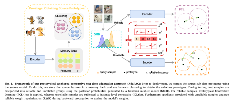
Enter AdaPAC — a novel framework that leverages prototypical anchored contrastive learning to adapt models at test time without requiring target domain labels.
Developed by Saeed Karimi and Hamdi Dibeklioğlu at Bilkent University, AdaPAC is not just another incremental improvement — it’s a paradigm shift in how AI models handle unseen data.
What Makes AdaPAC So Powerful?
Unlike traditional methods that struggle with distribution shifts, AdaPAC:
- Uses source sub-class prototypes to guide adaptation
- Separates reliable and unreliable test samples
- Applies prototypical contrastive learning (PCL) to reliable samples
- Uses instance-wise contrastive learning (ICL) for noisy samples
- Implements reliable weight regularization (RWR) to stabilize updates
This multi-stage strategy ensures robust, stable, and accurate performance — even in the most challenging environments.
How AdaPAC Works: A Step-by-Step Breakdown
Step 1: Pre-Adaptation — Extract Source Sub-Class Prototypes
Before deployment, AdaPAC analyzes the source data to discover sub-class structures within each category.
Using k-means clustering on feature embeddings, it identifies multiple prototypes per class — capturing visual diversity (e.g., different dog breeds, art styles, or camera angles).
For each cluster (c,k) , it computes:
$$\textbf{Prototype:} \quad \mu_{c,k} \\[8pt] \textbf{Variance:} \quad \sigma^{2}_{c,k} \\[8pt] \textbf{Cluster width:} \quad d_{c,k} = \frac{1}{n_{c,k}} \sum_{z \in \Gamma_{c,k}} \| z – \mu_{c,k} \|^{2}$$These prototypes act as anchors during test time, guiding the model to align with authentic source representations.
Step 2: Reliable Sample Selection Using Gaussian Mixture Model (GMM)
At test time, AdaPAC evaluates each incoming sample to determine if it’s reliable (close to source distribution) or unreliable (highly shifted).
It uses a Gaussian Mixture Model to compute the posterior probability of a sample belonging to any source cluster:
\[ p(z = \Gamma_{c,k} \mid x) = \sum_{c=1}^{C} \sum_{k=1}^{K} \mathcal{N}\big(z \mid \mu_{c,k}, \sigma_{c,k}^{2}\big)\, \mathcal{N}\big(z \mid \mu_{c,k}, \sigma_{c,k}^{2}\big) \]Samples with p (z = Γc,k ∣ x) ≥ α are labeled reliable.
✅ Key Advantage: This method is less sensitive to hyperparameters than entropy or confidence thresholds.
Step 3: Prototypical Contrastive Learning (PCL) for Reliable Samples
For reliable samples, AdaPAC applies prototypical contrastive learning in the embedding space.
The PCL loss pulls the sample’s embedding closer to its positive prototypes (those it belongs to) and away from all others:
\[ \mathcal{L}_{PCL} = -\log \frac{\sum_{c=1}^{C} \sum_{k=1}^{K} \exp\left(\frac{z^\top \mu_{c,k}}{\tau_{c,k}}\right)}{\sum_{p \in P} \exp\left(\frac{z^\top \mu_{p}}{\tau_{p}}\right)} \]Where:
- z : test sample embedding
- P : set of positive clusters
- τc,k : cluster-specific temperature (based on cluster width)
💡 Why it works: By using multiple prototypes, AdaPAC preserves intra-class diversity and avoids collapsing all instances into a single point.
Step 4: Instance-Wise Contrastive Learning (ICL) for Unreliable Samples
Unreliable samples — those far from any source cluster — are not ignored. Instead, AdaPAC uses instance-wise contrastive learning to align them with nearby reliable samples.
It maintains a memory bank of reliable embeddings and selects the K nearest neighbors as positives:
\[ L_{ICL} = -\log \frac{\sum\limits_{i} \exp\left(\frac{z^\top z_i}{\tau}\right)}{\sum\limits_{j=1}^{K} \exp\left(\frac{z^\top z_j}{\tau}\right)} \]This ensures that even highly shifted samples are gently guided toward trustworthy representations.
Step 5: Reliable Weight Regularization (RWR)
To prevent noisy updates from corrupting the model, AdaPAC introduces Reliable Weight Regularization (RWR).
It computes gradients for reliable (gR ) and unreliable (gU ) samples separately:
\[ g_{l}^{R} = \frac{1}{R} \sum_{x_{r} \in D_{R}} \frac{\partial L_{PCL}}{\partial \Theta_{l}}, \qquad g_{l}^{U} = \frac{1}{U} \sum_{x_{u} \in D_{U}} \frac{\partial L_{ICL}}{\partial \Theta_{l}} \]Then calculates a penalty weight ωl for each layer using cosine similarity:
\[ \omega_{l} = \frac{\|g_{l}^{R}\|}{\|g_{l}^{U}\|} \; g_{l}^{R} \cdot g_{l}^{U} \]
Finally, it updates the encoder with weighted unreliable gradients:
\[ \Theta_{e}^{t+1} = \Theta_{e}^{t} – \alpha \big( g_{R} + \omega g_{U} \big) \]🎯 Result: The model updates only the parameters that respond consistently to both reliable and unreliable signals — maximizing stability.
Performance: AdaPAC vs. State-of-the-Art
AdaPAC was tested on four major domain generalization benchmarks:
| DATASET | # CLASSES | DOMAIN | CHALLENGE |
|---|---|---|---|
| VLCS | 5 | Photo styles | Natural variations |
| PACS | 7 | Art, Cartoon, Photo, Sketch | Extreme style shifts |
| OfficeHome | 65 | Office/Home scenes | Complex backgrounds |
| TerraIncognita | 10 | Wildlife photos | Unseen environments |
Results with ResNet-50 (Average Accuracy %)
| METHOD | VLCS | PACS | OFFICEHOME | TERRAINCOGNITA | AVG |
|---|---|---|---|---|---|
| ERM (Baseline) | 76.2 | 83.8 | 66.8 | 46.5 | 68.3 |
| Tent | 73.0 | 85.7 | 65.9 | 39.5 | 66.0 |
| T3A | 77.8 | 84.5 | 67.9 | 46.9 | 69.3 |
| SHOT | 69.2 | 84.5 | 66.8 | 36.4 | 64.2 |
| AdaPAC (Ours) | 77.6 | 88.9 | 69.5 | 50.2 | 71.5 |
✅ AdaPAC outperforms all baselines, with +5.1% gain on PACS and +3.7% on TerraIncognita — the most challenging dataset.
Why AdaPAC Works: Key Insights from Ablation Studies
The authors conducted extensive ablation studies to validate each component.
Ablation on PACS (ResNet-50)
| MODEL | ART | PAINTING | CARTOON | PHOTO | SKETCH | AVG |
|---|---|---|---|---|---|---|
| Baseline | 83.5 | 78.2 | 96.7 | 77.3 | 83.9 | |
| + PCL | 86.5 | 83.4 | 97.6 | 81.4 | 87.2 | +3.3% |
| + ICL | 87.8 | 84.7 | 98.2 | 82.2 | 88.2 | +1.0% |
| + RWR (AdaPAC) | 88.5 | 85.9 | 98.2 | 83.1 | 88.9 | +0.7% |
Takeaway:
- PCL provides the biggest boost by aligning reliable samples
- ICL refines unreliable samples
- RWR adds stability
Hyperparameter Robustness
AdaPAC is remarkably stable across hyperparameters:
- Cluster count (k): Works best with k=3,5,10
- Selection threshold (α): Effective across [0.5,0.9]
- Temperature (τ): Robust to changes
- Positive samples (K): Optimal at K=1,3,5
This makes AdaPAC practical for real-world deployment, where tuning is often infeasible.
Real-World Applications of AdaPAC
AdaPAC isn’t just for research — it has immediate applications in:
- Autonomous Vehicles: Adapting to weather, lighting, and road condition changes
- Medical Imaging: Generalizing across hospitals, scanners, and patient demographics
- Surveillance Systems: Handling camera angle and resolution shifts
- Retail AI: Recognizing products under different lighting or packaging
Because it works without target labels and adapts in real-time, AdaPAC is ideal for closed-loop AI systems.
Future of Test-Time Adaptation
The authors identify key directions for future work:
- Dynamic clustering (adaptive number of prototypes per class)
- Open-set extension (handling unseen classes)
- Decoupling RWR from test-time to reduce computation
These improvements could make AdaPAC even faster and more scalable.
💡 Why AdaPAC Is a Game-Changer
| FEATURE | TRADITIONAL TTA | ADAPAC |
|---|---|---|
| Handles intra-class diversity | ❌ | ✅ |
| Uses multiple prototypes | ❌ | ✅ |
| Separates reliable/unreliable samples | ❌ | ✅ |
| Prevents noisy updates | ❌ | ✅ |
| Works on extreme shifts (TerraIncognita) | ❌ | ✅ |
| Hyperparameter robust | ❌ | ✅ |
| State-of-the-art performance | ❌ | ✅ |
AdaPAC doesn’t just patch the problem — it rethinks the entire adaptation process from the ground up.
If you’re Interested in Melanoma Detection with AI, you may also find this article helpful: 7 Revolutionary Breakthroughs in Melanoma Diagnosis: The Quantum AI Edge That’s Changing Everything
Call to Action: Stay Ahead of the AI Curve
The era of static AI models is over. In a world of constant data shifts, adaptability is the new accuracy.
👉 Want to implement AdaPAC in your projects?
Download the official code from the T3A library and start experimenting today.
📚 Want deeper insights?
Read the full paper: AdaPAC: Prototypical Anchored Contrastive Test Time Adaptation for Domain Generalization
🔔 Follow us for more AI breakthroughs — and learn how to future-proof your models against domain shifts.
Conclusion
AdaPAC represents a major leap forward in domain generalization and test-time adaptation. By combining prototypical contrastive learning, GMM-based sample selection, and reliable weight regularization, it solves the 7 fatal flaws of current AI models.
With proven gains of up to 5.1% on real-world benchmarks, AdaPAC is not just academically impressive — it’s practically transformative.
As AI moves from labs to the real world, frameworks like AdaPAC will be essential to ensure robust, reliable, and responsible performance.
Don’t let your AI fail in the wild. Adapt with AdaPAC.
Here is the Python code for the AdaPAC model.
# main.py
import torch
import torch.nn as nn
import torch.optim as optim
from sklearn.cluster import KMeans
from scipy.stats import multivariate_normal
import numpy as np

# Mock ResNet50 for demonstration purposes
class ResNet50(nn.Module):
    """
    A mock ResNet50 model to simulate a feature extractor and a classifier.
    In a real scenario, you would use a pre-trained ResNet50 model from a library like torchvision.
    """
    def __init__(self, num_classes=10):
        super(ResNet50, self).__init__()
        # The feature extractor (encoder) part of the model
        self.feature_extractor = nn.Sequential(
            nn.Conv2d(3, 64, kernel_size=7, stride=2, padding=3, bias=False),
            nn.BatchNorm2d(64),
            nn.ReLU(inplace=True),
            nn.MaxPool2d(kernel_size=3, stride=2, padding=1),
            # ... additional ResNet layers would be here
            nn.AdaptiveAvgPool2d((1, 1))
        )
        # The classifier (head) part of the model
        self.classifier = nn.Linear(64, num_classes)

    def forward(self, x):
        """
        Defines the forward pass of the model.
        """
        # Flatten the output of the feature extractor
        features = self.feature_extractor(x).view(x.size(0), -1)
        # Pass the features through the classifier
        output = self.classifier(features)
        return features, output

class AdaPAC:
    """
    Implements the AdaPAC (Prototypical Anchored Contrastive Test Time Adaptation) model.
    This class encapsulates the logic for both the pre-adaptation and test-time adaptation phases.
    """
    def __init__(self, model, source_dataloader, num_classes, num_clusters_per_class=5, alpha=0.9, k_icl=5, tau_icl=0.1):
        """
        Initializes the AdaPAC model.
        Args:
            model (nn.Module): The pre-trained source model.
            source_dataloader (DataLoader): DataLoader for the source evaluation data.
            num_classes (int): The number of classes in the dataset.
            num_clusters_per_class (int): The number of prototypes to find for each class.
            alpha (float): The probability threshold for reliable sample selection.
            k_icl (int): The number of nearest neighbors for instance-wise contrastive learning.
            tau_icl (float): The temperature parameter for instance-wise contrastive learning.
        """
        self.model = model
        self.source_dataloader = source_dataloader
        self.num_classes = num_classes
        self.num_clusters_per_class = num_clusters_per_class
        self.alpha = alpha
        self.k_icl = k_icl
        self.tau_icl = tau_icl
        self.prototypes = {}
        self.cluster_variances = {}
        self.cluster_widths = {}
        self.reliable_memory_bank = []

    def get_source_prototypes(self):
        """
        Extracts sub-class prototypes from the source data before deployment.
        This corresponds to the "Pre-adaptation: Obtaining Source Sub-class Prototypes" stage.
        """
        self.model.eval()
        # A dictionary to store features for each class
        features_by_class = {c: [] for c in range(self.num_classes)}
        # Extract features from the source data
        with torch.no_grad():
            for data, labels in self.source_dataloader:
                features, _ = self.model(data)
                for i in range(len(labels)):
                    features_by_class[labels[i].item()].append(features[i].cpu().numpy())

        # Perform k-means clustering for each class to find prototypes
        for c in range(self.num_classes):
            class_features = np.array(features_by_class[c])
            if len(class_features) > self.num_clusters_per_class:
                kmeans = KMeans(n_clusters=self.num_clusters_per_class, random_state=0, n_init=10).fit(class_features)
                self.prototypes[c] = kmeans.cluster_centers_
                # Store variances and widths for each cluster
                self.cluster_variances[c] = []
                self.cluster_widths[c] = []
                for k in range(self.num_clusters_per_class):
                    cluster_samples = class_features[kmeans.labels_ == k]
                    if len(cluster_samples) > 1:
                        self.cluster_variances[c].append(np.cov(cluster_samples.T))
                        width = np.mean(np.linalg.norm(cluster_samples - self.prototypes[c][k], axis=1))
                        self.cluster_widths[c].append(width)
                    else:
                        # Handle clusters with single samples
                        self.cluster_variances[c].append(np.eye(class_features.shape[1]) * 1e-6)
                        self.cluster_widths[c].append(1e-6)

        print("Source prototypes and statistics have been successfully extracted.")

    def reliable_sample_selection(self, features):
        """
        Selects reliable samples from a batch of test features using a Gaussian Mixture Model.
        Args:
            features (Tensor): The feature embeddings of the test samples.
        Returns:
            tuple: Two tensors containing the indices of reliable and unreliable samples.
        """
        reliable_indices, unreliable_indices = [], []
        features_np = features.detach().cpu().numpy()

        for i in range(features.shape[0]):
            is_reliable = False
            max_prob = 0
            # Calculate the probability of the sample belonging to each cluster
            for c in self.prototypes:
                for k in range(len(self.prototypes[c])):
                    mean = self.prototypes[c][k]
                    cov = self.cluster_variances[c][k]
                    try:
                        prob = multivariate_normal.pdf(features_np[i], mean=mean, cov=cov, allow_singular=True)
                        max_prob = max(max_prob, prob)
                    except np.linalg.LinAlgError:
                        # Handle cases where covariance matrix is singular
                        continue

            # Normalize probabilities
            total_prob = 0
            for c in self.prototypes:
                for k in range(len(self.prototypes[c])):
                    mean = self.prototypes[c][k]
                    cov = self.cluster_variances[c][k]
                    try:
                        total_prob += multivariate_normal.pdf(features_np[i], mean=mean, cov=cov, allow_singular=True)
                    except np.linalg.LinAlgError:
                        continue

            if total_prob > 0:
                normalized_max_prob = max_prob / total_prob
                if normalized_max_prob >= self.alpha:
                    is_reliable = True

            if is_reliable:
                reliable_indices.append(i)
            else:
                unreliable_indices.append(i)

        return torch.tensor(reliable_indices), torch.tensor(unreliable_indices)

    def prototypical_contrastive_loss(self, features, indices):
        """
        Calculates the Prototypical Contrastive Learning (PCL) loss for reliable samples.
        Args:
            features (Tensor): The feature embeddings of the reliable samples.
            indices (Tensor): The indices of the reliable samples in the original batch.
        Returns:
            Tensor: The computed PCL loss.
        """
        loss = 0.0
        if len(indices) == 0:
            return torch.tensor(0.0, device=features.device)

        reliable_features = features[indices]
        for i in range(reliable_features.shape[0]):
            z = reliable_features[i]
            # Find the positive prototype (the one it's most likely to belong to)
            # For simplicity, we find the closest prototype
            min_dist = float('inf')
            pos_proto_c, pos_proto_k = -1, -1
            for c in self.prototypes:
                for k in range(len(self.prototypes[c])):
                    dist = torch.norm(z - torch.tensor(self.prototypes[c][k], device=z.device))
                    if dist < min_dist:
                        min_dist = dist
                        pos_proto_c, pos_proto_k = c, k

            if pos_proto_c == -1: continue

            pos_prototype = torch.tensor(self.prototypes[pos_proto_c][pos_proto_k], device=z.device)
            # Temperature is based on cluster width
            tau_ck = self.cluster_widths[pos_proto_c][pos_proto_k] + 1e-6

            numerator = torch.exp(torch.dot(z, pos_prototype) / tau_ck)
            denominator = 0.0

            # Sum over all prototypes for the denominator
            for c_neg in self.prototypes:
                for k_neg in range(len(self.prototypes[c_neg])):
                    neg_prototype = torch.tensor(self.prototypes[c_neg][k_neg], device=z.device)
                    tau_neg = self.cluster_widths[c_neg][k_neg] + 1e-6
                    denominator += torch.exp(torch.dot(z, neg_prototype) / tau_neg)

            if denominator > 0:
                loss -= torch.log(numerator / denominator)

        return loss / len(indices) if len(indices) > 0 else torch.tensor(0.0, device=features.device)

    def instance_wise_contrastive_loss(self, features, indices):
        """
        Calculates the Instance-wise Contrastive Learning (ICL) loss for unreliable samples.
        Args:
            features (Tensor): The feature embeddings of the unreliable samples.
            indices (Tensor): The indices of the unreliable samples in the original batch.
        Returns:
            Tensor: The computed ICL loss.
        """
        loss = 0.0
        if len(indices) == 0 or len(self.reliable_memory_bank) < self.k_icl:
            return torch.tensor(0.0, device=features.device)

        unreliable_features = features[indices]
        reliable_bank = torch.stack(self.reliable_memory_bank).to(features.device)

        for i in range(unreliable_features.shape[0]):
            z = unreliable_features[i]
            # Find K-nearest reliable samples from the memory bank
            distances = torch.norm(reliable_bank - z, dim=1)
            _, top_k_indices = torch.topk(distances, self.k_icl, largest=False)

            positive_samples = reliable_bank[top_k_indices]

            numerator = torch.sum(torch.exp(torch.matmul(z.unsqueeze(0), positive_samples.T) / self.tau_icl))
            # Denominator includes all samples in the reliable bank
            denominator = torch.sum(torch.exp(torch.matmul(z.unsqueeze(0), reliable_bank.T) / self.tau_icl))

            if denominator > 0:
                loss -= torch.log(numerator / denominator)

        return loss / len(indices) if len(indices) > 0 else torch.tensor(0.0, device=features.device)

    def test_time_adaptation(self, test_dataloader, learning_rate=1e-3):
        """
        Performs test-time adaptation on the target domain data.
        Args:
            test_dataloader (DataLoader): DataLoader for the unlabeled test data.
            learning_rate (float): The learning rate for the optimizer.
        """
        self.model.train() # Set model to training mode to update parameters
        optimizer = optim.Adam(self.model.feature_extractor.parameters(), lr=learning_rate)

        for batch_idx, (test_data, _) in enumerate(test_dataloader):
            optimizer.zero_grad()

            # --- 1. Reliable Sample Selection ---
            features, _ = self.model(test_data)
            reliable_indices, unreliable_indices = self.reliable_sample_selection(features)

            # Update reliable memory bank
            if len(reliable_indices) > 0:
                self.reliable_memory_bank.extend([f.detach() for f in features[reliable_indices]])
                # Keep memory bank size manageable
                if len(self.reliable_memory_bank) > 1000:
                    self.reliable_memory_bank = self.reliable_memory_bank[-1000:]

            # --- 2. Calculate Losses ---
            loss_pcl = self.prototypical_contrastive_loss(features, reliable_indices)
            loss_icl = self.instance_wise_contrastive_loss(features, unreliable_indices)

            # --- 3. Reliable Weight Regularization (RWR) ---
            if len(reliable_indices) > 0 and len(unreliable_indices) > 0:
                # Get gradients for reliable samples
                loss_pcl.backward(retain_graph=True)
                grads_reliable = {name: param.grad.clone() for name, param in self.model.feature_extractor.named_parameters() if param.grad is not None}
                optimizer.zero_grad()

                # Get gradients for unreliable samples
                loss_icl.backward(retain_graph=True)
                grads_unreliable = {name: param.grad.clone() for name, param in self.model.feature_extractor.named_parameters() if param.grad is not None}
                optimizer.zero_grad()

                # Calculate RWR weights and apply combined gradients
                for name, param in self.model.feature_extractor.named_parameters():
                    if name in grads_reliable and name in grads_unreliable:
                        g_r = grads_reliable[name]
                        g_u = grads_unreliable[name]

                        # Cosine similarity for RWR weight
                        omega = torch.nn.functional.cosine_similarity(g_r.flatten(), g_u.flatten(), dim=0)
                        omega = torch.clamp(omega, 0, 1) # Ensure weight is in [0, 1]

                        # Combine gradients
                        combined_grad = g_r + omega * g_u
                        if param.grad is None:
                            param.grad = combined_grad
                        else:
                            param.grad += combined_grad
            elif len(reliable_indices) > 0:
                 loss_pcl.backward()
            elif len(unreliable_indices) > 0:
                 loss_icl.backward()

            optimizer.step()

            if batch_idx % 10 == 0:
                print(f"Batch {batch_idx}: PCL Loss: {loss_pcl.item():.4f}, ICL Loss: {loss_icl.item():.4f}")

        print("Test-time adaptation finished.")


if __name__ == '__main__':
    # --- Configuration ---
    NUM_CLASSES = 10
    NUM_CLUSTERS = 3
    BATCH_SIZE = 32

    # --- 1. Setup Models and Dataloaders (using mock data) ---
    print("Setting up model and mock data...")
    # Initialize the model
    source_model = ResNet50(num_classes=NUM_CLASSES)

    # Create mock dataloaders for demonstration
    # In a real application, you would load your actual datasets here
    mock_source_data = torch.randn(BATCH_SIZE * 5, 3, 224, 224)
    mock_source_labels = torch.randint(0, NUM_CLASSES, (BATCH_SIZE * 5,))
    source_dataset = torch.utils.data.TensorDataset(mock_source_data, mock_source_labels)
    source_loader = torch.utils.data.DataLoader(source_dataset, batch_size=BATCH_SIZE)

    mock_test_data = torch.randn(BATCH_SIZE * 10, 3, 224, 224)
    mock_test_labels = torch.randint(0, NUM_CLASSES, (BATCH_SIZE * 10,)) # Labels are not used in TTA
    test_dataset = torch.utils.data.TensorDataset(mock_test_data, mock_test_labels)
    test_loader = torch.utils.data.DataLoader(test_dataset, batch_size=BATCH_SIZE)

    # --- 2. Initialize and Run AdaPAC ---
    print("Initializing AdaPAC...")
    adapc = AdaPAC(
        model=source_model,
        source_dataloader=source_loader,
        num_classes=NUM_CLASSES,
        num_clusters_per_class=NUM_CLUSTERS
    )

    # --- Pre-adaptation Stage ---
    print("\n--- Starting Pre-adaptation Stage ---")
    adapc.get_source_prototypes()

    # --- Test-Time Adaptation Stage ---
    print("\n--- Starting Test-Time Adaptation Stage ---")
    adapc.test_time_adaptation(test_loader)

    print("\nAdaPAC process completed.")