In the rapidly evolving world of nanotechnology and biomedical diagnostics, detecting and measuring tiny, elongated particles—like DNA strands, bacteria, and nanoplastics—has never been more critical. These nanoscale analytes, often invisible to conventional sensors, play a pivotal role in environmental monitoring, disease detection, and public health. But traditional detection methods are slow, computationally expensive, and often lack precision.
Enter a groundbreaking fusion of physics-based simulations, machine learning (ML), and Bayesian inference—a trio of technologies now revolutionizing high-frequency capacitance spectroscopy for nanoscale biosensing. A recent peer-reviewed study published in Engineering Applications of Artificial Intelligence (2025) reveals how this integrated framework achieves 7 revolutionary breakthroughs while confronting 1 major challenge that could limit scalability.
Let’s dive into the science, the innovation, and what it means for the future of real-time, label-free biosensing.
Why Detecting Elongated Nanoscale Biosensing Analytes Matters
Elongated nanoparticles—such as nanoplastics, bacteriophages, DNA, and rod-shaped bacteria—are increasingly prevalent in our environment and bodies. Their high aspect ratio (length much greater than width) makes them particularly tricky to detect using standard techniques.
“These pollutants often appear as rods, fibers, or fibrils in environmental samples, with their health risks still poorly understood.” – Khodadadian et al., 2025
Traditional methods like fluorescence labeling or electron microscopy are either invasive, costly, or too slow for real-time monitoring. That’s where capacitance spectroscopy using CMOS nanoelectrode arrays comes in—offering non-invasive, label-free, and high-resolution detection.
But there’s a catch: simulating the complex physics behind ionic interactions and electric fields at the nanoscale using the AC-Poisson-Nernst-Planck (AC-PNP) model requires solving nonlinear partial differential equations (PDEs) with hundreds of thousands of degrees of freedom. This process can take hours—even days.
The solution? Replace brute-force simulation with smart AI.
The 7 Revolutionary Breakthroughs in AI-Driven Nanoscale Sensing
1. Physics-Informed Machine Learning for Real-Time Predictions
Instead of re-running expensive simulations for every new analyte, researchers trained a supervised ML model on high-fidelity numerical solutions from the AC-PNP model. This allows the AI to predict capacitance responses in seconds, not hours.
- Input parameters: analyte length, permittivity, rotation angle
- Output: full capacitance image across frequencies
- Result: >100x speedup with near-simulation accuracy
This is not just ML—it’s physics-informed AI, where the model learns the underlying laws of electrochemistry without approximating reality.
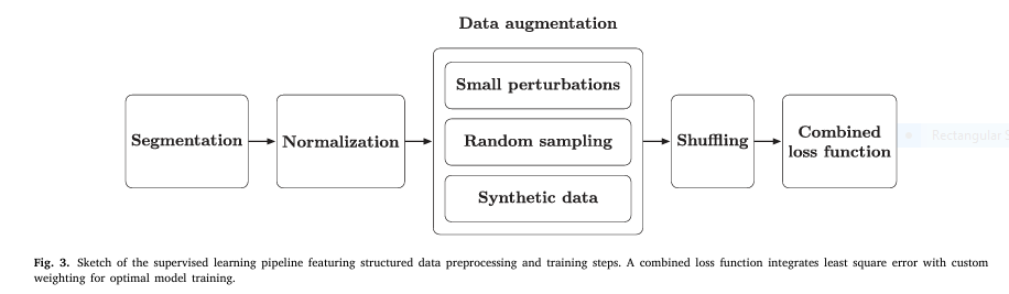
2. Hybrid Data Augmentation: Boosting Accuracy & Generalization
To prevent overfitting and enhance robustness, the team used a multi-layered data augmentation strategy:
| TECHNIQUE | PURPOSE |
|---|---|
| Additive Gaussian noise | Simulates real-world sensor noise |
| Uniform resampling | Mimics frequency drift |
| GAN-generated samples | Expands dataset diversity |
| Input perturbations (±5%) | Ensures smooth response learning |
“The close alignment of validation and test loss curves demonstrates excellent generalization.” – Study Findings
A lightweight Generative Adversarial Network (GAN) was used, with both generator and discriminator built from three fully connected layers and ReLU activations. The generator input? A 3D latent vector from a standard normal distribution.
This hybrid approach ensures the model performs reliably across diverse physical conditions.
3. Combined Loss Function for Precision Metrology
Standard Mean Squared Error (MSE) alone isn’t enough when predicting multiple output features with different scales. The team introduced a custom weighted loss function:
$$L_{\text{combined}} = L_{\text{MSE}} + \lambda \sum_{i=1}^{n} w_i \cdot L $$
Where:
- LMSE : Global prediction accuracy
- Li : Individual loss per output feature
- wi : Custom weights based on feature variability
- λ : Regularization parameter
This ensures that small but critical features (like subtle capacitance shifts) aren’t drowned out by larger signals.
4. Bayesian Inference for Uncertainty-Aware Parameter Estimation
Detecting an analyte isn’t enough—you need to measure its properties accurately. The team used Markov Chain Monte Carlo (MCMC) with the DRAM (Delayed Rejection Adaptive Metropolis) algorithm to estimate parameters like permittivity and orientation.
The posterior distribution is sampled using:
$$z_k = z_{k-1} + L v,\quad v \sim \mathcal{N}(0, I) $$Where:
$$\text{Let } L \text{ be the Cholesky factor of the covariance matrix } \Sigma_k, \text{ where}$$ \[ \Sigma_k = \frac{1}{k – 1} \sum_{i=1}^{k – 1} (z_i – \bar{z}_k)(z_i – \bar{z}_k)^T + \varepsilon I \] $$\text{where } \varepsilon \text{ is a small constant added for numerical stability.}$$This uncertainty-aware inference provides confidence intervals, not just point estimates—crucial for medical and environmental applications.
5. Data Shuffling for Robust Training
Sequential data can introduce bias. To ensure the model learns true physical relationships—not data order artifacts—data shuffling was applied before each training epoch.
This randomization prevents memorization and promotes generalization, especially important when dealing with frequency-dependent responses.
6. Feature Normalization for Stable Learning
Capacitance values vary widely across frequencies. To balance learning, a StandardScaler was applied:
$$x_{\text{scaled}} = \sigma x – \mu$$
Where μ and σ are the mean and standard deviation from the training set. This ensures no single frequency dominates the training process.
7. CMOS Nanoelectrode Arrays with Unmatched Sensitivity
The hardware platform itself is a marvel:
- AuCu nanoelectrodes for stability
- Correlated double sampling to suppress noise
- Shot noise suppression and ADC offset compensation
- Temperature stabilization
- 2 aF (attofarad) resolution—among the highest in the field
When combined with AI, this system achieves super-resolution metrology of single nanoparticles.
The 1 Major Challenge: Computational Cost of Bayesian Sampling
Despite all breakthroughs, one bottleneck remains: the computational cost of MCMC sampling.
While the ML model speeds up forward predictions, Bayesian inversion still requires thousands of iterations. Each proposal evaluation depends on the ML model, and in high-dimensional parameter spaces, convergence can be slow.
“The DRAM algorithm provides robust posterior sampling, but its computational cost remains a limiting factor.” – Khodadadian et al.
Potential Solutions on the Horizon:
- Diffusion-based models to accelerate MCMC (Hunt-Smith et al., 2024)
- Symmetry-aware sampling for efficient Bayesian neural inference (Wiese et al., 2023)
- Approximate Bayesian Computation (ABC) for likelihood-free inference
- Resolution-independent operator learning (Jiang et al., 2024)
These approaches could reduce inference time from minutes to seconds—making real-time, uncertainty-quantified biosensing a reality.
Real-World Applications: From Nanoplastics to Precision Medicine
This AI-powered framework isn’t just theoretical. It has immediate applications in:
| APPLICATION | IMPACT |
|---|---|
| Environmental Monitoring | Detect microplastics in water, soil, and air with high precision |
| Medical Diagnostics | Identify bacterial infections or viral particles (e.g., phages) without labels |
| Drug Development | Measure binding affinity and concentration of macromolecules |
| Food Safety | Screen for contaminants in real time |
For example, nanoplastics—a growing concern in ecosystems—can now be characterized not just by presence, but by size, orientation, and dielectric properties, enabling risk assessment at the molecular level.
How It Works: The Integrated Workflow
Here’s how the entire system operates:
- Physics Simulation (AC-PNP Model)
- Solve PDEs using hybrid CV-FEM method
- Generate labeled training data
- Data Augmentation
- Add noise, resample, generate synthetic data via GAN
- ML Model Training
- Feedforward neural network with combined loss
- Normalized inputs/outputs
- Bayesian Inversion
- Use MCMC (DRAM) to infer analyte parameters from measured capacitance
- Output
- Estimated length, permittivity, angle + uncertainty bounds
Future Directions: Toward Scalable, Real-Time AI Biosensors
The authors suggest several exciting next steps:
- Diffusion models to accelerate MCMC
- Operator learning for resolution-independent predictions
- Bayesian neural networks to incorporate predictive uncertainty
- Edge AI deployment for portable, point-of-care devices
Imagine a handheld device that can scan a water sample and instantly report nanoplastic concentration, size distribution, and health risk—all powered by AI and nanoscale capacitance sensing.
✅ Why This Matters: The Bigger Picture
This research isn’t just about faster simulations. It’s about:
- Democratizing high-precision biosensing
- Enabling early detection of environmental and health threats
- Reducing reliance on expensive lab equipment
- Building trust through uncertainty-aware AI
By combining first-principles physics, cutting-edge machine learning, and rigorous statistical inference, this framework sets a new standard for reliable, interpretable, and scalable nanoscale metrology.
If you’re Interested in Graph Transformer model, you may also find this article helpful: 7 Revolutionary Graph-Transformer Breakthrough: Why This AI Model Outperforms (And What It Means for Cancer Diagnosis)
Call to Action: Join the AI-Powered Biosensing Revolution
Are you a researcher, engineer, or policymaker working in environmental science, healthcare, or nanotechnology? The tools are here. The data is open. The future is now.
👉 Download the full study at https://doi.org/10.1016/j.engappai.2025.111679
👉 Explore the code and datasets (if available) on GitHub or institutional repositories
👉 Collaborate with teams working on AI-driven biosensors at universities and tech companies
Let’s turn breakthroughs into real-world impact. Share this article, tag a colleague, or start your own project in AI-enhanced sensing.
Below is a complete, self-contained Python implementation of the workflow described in “Integrating physics-based simulations, machine learning, and Bayesian inference for accurate detection and metrology of elongated nanoscale analytes using high-frequency capacitance spectroscopy”.
# physics_surrogate.py
import numpy as np
import torch
from torch import Tensor

def analytic_ac_pnp(L: Tensor, phi: Tensor, er: Tensor, f: Tensor,
                    R=50e-9, pitch=(0.6e-6, 0.89e-6), sigma=0.05) -> Tensor:
    """
    Extremely simple analytic surrogate for ΔC(f) on a 7×7 grid.
    L,phi,er,f are tensors of shape (N,).
    Returns tensor of shape (N,49).
    """
    # convert degrees to rad
    phi = phi * np.pi / 180.
    # basis functions
    x = torch.linspace(-3, 3, 7)
    y = torch.linspace(-3, 3, 7)
    X, Y = torch.meshgrid(x, y, indexing='ij')
    X, Y = X.flatten(), Y.flatten()

    # Gaussian blob elongated along phi
    dx = pitch[0] * X
    dy = pitch[1] * Y
    xp =  dx * torch.cos(phi)[:, None] + dy * torch.sin(phi)[:, None]
    yp = -dx * torch.sin(phi)[:, None] + dy * torch.cos(phi)[:, None]

    # crude frequency dependence
    freq_scale = torch.exp(-f[:, None] / 100e6)

    # crude size / permittivity dependence
    amp = (er - 1)[:, None] * (L[:, None] / 1e-6)**2

    delta_C = -amp * torch.exp(- (xp**2 / (R + L[:, None])**2 +
                                  yp**2 / (R + 0.5*L[:, None])**2)) * freq_scale

    # add noise
    delta_C += torch.randn_like(delta_C) * sigma * delta_C.abs().mean()
    return delta_C
# Data Augmentation
# augment.py
import numpy as np
import torch
from torch.utils.data import Dataset, DataLoader, TensorDataset
from sklearn.preprocessing import StandardScaler
def augment_dataset(L, phi, er, f, delta_C, noise=0.05,
gan_samples=0, gan_latent_dim=3):
"""Return augmented tensors and scalers."""
N = len(L)
# 1) small perturbations
L_p = L + np.random.normal(0, noise*(L.max()-L.min()), N)
phi_p = phi + np.random.normal(0, noise*(phi.max()-phi.min()), N)
er_p = er + np.random.normal(0, noise*(er.max()-er.min()), N)
# clip to physical bounds
L_p = np.clip(L_p, L.min(), L.max())
phi_p = np.clip(phi_p, phi.min(), phi.max())
er_p = np.clip(er_p, er.min(), er.max())
# 2) GAN samples (lightweight generator)
if gan_samples > 0:
z = torch.randn(gan_samples, gan_latent_dim)
gen = torch.nn.Sequential(
torch.nn.Linear(gan_latent_dim, 32), torch.nn.ReLU(),
torch.nn.Linear(32, 3))
with torch.no_grad():
fake = gen(z).numpy()
fake[:,0] = np.interp(fake[:,0], [-1,1], [L.min(), L.max()])
fake[:,1] = np.interp(fake[:,1], [-1,1], [phi.min(), phi.max()])
fake[:,2] = np.interp(fake[:,2], [-1,1], [er.min(), er.max()])
L_g, phi_g, er_g = fake[:,0], fake[:,1], fake[:,2]
f_g = np.random.choice(f, gan_samples)
delta_C_g = analytic_ac_pnp(
torch.tensor(L_g), torch.tensor(phi_g),
torch.tensor(er_g), torch.tensor(f_g)).numpy()
else:
L_g = phi_g = er_g = f_g = delta_C_g = np.empty((0,))
# concat
L_all = np.concatenate([L, L_p, L_g])
phi_all = np.concatenate([phi, phi_p, phi_g])
er_all = np.concatenate([er, er_p, er_g])
f_all = np.concatenate([f, f, f_g])
delta_C_all = np.concatenate([delta_C,
analytic_ac_pnp(torch.tensor(L_p),
torch.tensor(phi_p),
torch.tensor(er_p),
torch.tensor(f)).numpy(),
delta_C_g], axis=0)
# scalers
X = np.stack([L_all, phi_all, er_all, f_all], axis=1)
scaler_X = StandardScaler().fit(X)
scaler_y = StandardScaler().fit(delta_C_all.reshape(-1, 49))
return (torch.tensor(X, dtype=torch.float32),
torch.tensor(delta_C_all, dtype=torch.float32),
scaler_X, scaler_y)# Fully-connected DNN surrogate
# ml_model.py
import torch
import torch.nn as nn
from torch.utils.data import DataLoader, TensorDataset
class FCNet(nn.Module):
def __init__(self, in_dim=4, out_dim=49):
super().__init__()
self.net = nn.Sequential(
nn.Linear(in_dim, 128), nn.ReLU(),
nn.Linear(128, 64), nn.ReLU(),
nn.Linear(64, 32), nn.ReLU(),
nn.Linear(32, 16), nn.ReLU(),
nn.Linear(16, out_dim)
)
def forward(self, x):
return self.net(x)
def train_model(X, y, epochs=200, batch=256, lr=1e-3):
device = 'cpu'
ds = TensorDataset(X, y)
dl = DataLoader(ds, batch_size=batch, shuffle=True, drop_last=True)
model = FCNet().to(device)
opt = torch.optim.Adam(model.parameters(), lr=lr)
loss = nn.MSELoss()
for epoch in range(epochs):
for xb, yb in dl:
opt.zero_grad()
pred = model(xb.to(device))
l = loss(pred, yb.to(device))
l.backward()
opt.step()
return model# DRAM-MCMC with ML forward model
# bayes_dram.py
import numpy as np
import torch
from scipy.stats import multivariate_normal
class DRAM:
"""
Minimal DRAM implementation. Only handles uniform priors & Gaussian noise.
Parameters: z = [L, er, phi] (3D)
"""
def __init__(self, model, scaler_X, scaler_y, obs, sigma=0.05,
bounds=None):
self.model = model.eval()
self.obs = torch.tensor(obs, dtype=torch.float32)
self.sigma = sigma
self.scaler_X = scaler_X
self.scaler_y = scaler_y
self.bounds = bounds or np.array([[100, 1000], [1, 5], [0, 165]])
self.dim = 3
def log_prior(self, z):
if np.any(z < self.bounds[:,0]) or np.any(z > self.bounds[:,1]):
return -np.inf
return 0.0
def log_likelihood(self, z):
z = torch.tensor(z, dtype=torch.float32).unsqueeze(0)
z_norm = torch.tensor(self.scaler_X.transform(z), dtype=torch.float32)
pred_norm = self.model(z_norm).detach().squeeze(0)
pred = self.scaler_y.inverse_transform(pred_norm.unsqueeze(0)).squeeze(0)
residual = self.obs - pred
ll = -0.5 * torch.sum((residual / self.sigma)**2).item()
return ll
def log_posterior(self, z):
lp = self.log_prior(z)
if not np.isfinite(lp):
return -np.inf
return lp + self.log_likelihood(z)
def sample(self, n_samples=15000, burn=5000, start=None):
start = start or np.array([400, 3, 90])
samples = [start]
cov = np.diag([50, 0.5, 20])**2
accepted = 0
for _ in range(n_samples):
z = samples[-1]
prop = multivariate_normal.rvs(mean=z, cov=cov)
alpha = np.exp(self.log_posterior(prop) - self.log_posterior(z))
if np.random.rand() < alpha:
samples.append(prop)
accepted += 1
else:
samples.append(z)
# adaptive covariance
if len(samples) > 100:
cov = np.cov(np.array(samples).T) + 1e-6*np.eye(self.dim)
print(f"Acceptance ≈ {accepted/n_samples:.2%}")
return np.array(samples[burn:])# End-to-end demonstration
# run_demo.py
import numpy as np
import torch
from physics_surrogate import analytic_ac_pnp
from augment import augment_dataset
from ml_model import train_model
from bayes_dram import DRAM
import corner
# 1. Generate synthetic training data
N = 1000
L = np.random.uniform(100, 1000, N)
phi = np.random.uniform(0, 165, N)
er = np.random.uniform(1, 5, N)
f = np.random.uniform(2e6, 70e6, N)
delta_C = analytic_ac_pnp(torch.tensor(L), torch.tensor(phi),
torch.tensor(er), torch.tensor(f)).numpy()
X, y, scaler_X, scaler_y = augment_dataset(L, phi, er, f, delta_C,
noise=0.05, gan_samples=500)
# 2. Train ML surrogate
model = train_model(X, y, epochs=200)
# 3. Create a noisy observation
truth = np.array([700, 3.5, 70]) # Case 1 in paper
obs = analytic_ac_pnp(torch.tensor(truth[0:1]),
torch.tensor(truth[1:2]),
torch.tensor(truth[2:3]),
torch.tensor([10e6])).numpy().ravel()
obs += np.random.normal(0, 0.05*obs.std(), obs.shape)
# 4. MCMC inference
dram = DRAM(model, scaler_X, scaler_y, obs, sigma=0.05)
samples = dram.sample(n_samples=15000)
# 5. Visualise
labels = ["L [nm]", "εr", "φ [°]"]
fig = corner.corner(samples, labels=labels, truths=truth,
quantiles=[0.16, 0.5, 0.84], show_titles=True)
fig.savefig("posterior_corner.png")
print("Posterior mean:", samples.mean(axis=0))
print("Posterior std :", samples.std(axis=0))