BiMT-TCN: Revolutionizing Stock Price Prediction with Hybrid Deep Learning

In the fast-paced world of financial markets, accurate stock price prediction has long been the holy grail for investors, analysts, and AI researchers. With markets influenced by a complex web of economic indicators, geopolitical events, and investor sentiment, traditional models often fall short. Enter BiMT-TCN—a groundbreaking hybrid deep learning model that is redefining the accuracy and stability of stock market forecasts.

Published in the prestigious Knowledge-Based Systems journal, the BiMT-TCN model combines the strengths of Bidirectional LSTM (BiLSTM), a modified Transformer, and Temporal Convolutional Network (TCN) to deliver state-of-the-art performance across major global indices like the SSE, HSI, and NASDAQ. In this article, we’ll dive deep into how BiMT-TCN works, why it outperforms existing models, and what it means for the future of algorithmic trading and financial forecasting.

What Is BiMT-TCN? A Next-Gen Hybrid Model for Stock Prediction

The BiMT-TCN model stands for Bidirectional LSTM, Modified Transformer–Temporal Convolutional Network. It’s not just another deep learning architecture—it’s a purpose-built hybrid designed to overcome the limitations of individual models in capturing the multi-scale, non-linear, and volatile nature of financial time series.

Why Hybrid Models Matter in Finance

Stock price data is notoriously noisy, non-stationary, and influenced by both short-term fluctuations and long-term trends. No single deep learning model can optimally capture all these dynamics:

LSTMs are great at sequential learning but suffer from vanishing gradients over long sequences.
Transformers excel at modeling long-range dependencies but can lose fine-grained temporal precision.
TCNs are stable and efficient but may lack contextual depth.

BiMT-TCN solves this by strategically integrating all three:

BiLSTM captures bidirectional temporal dependencies.
Modified Transformer handles global context with enhanced attention.
TCN ensures robust, deep sequential pattern extraction with dilated convolutions.

This synergy allows BiMT-TCN to simultaneously model local volatility and global market trends—a critical advantage in real-world trading.

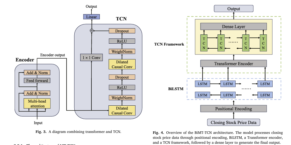
How BiMT-TCN Works: Architecture Breakdown

Let’s explore the BiMT-TCN architecture step by step, based on the research paper’s framework (Fig. 4).

1. Input & Positional Encoding

The model takes historical stock prices (e.g., closing prices) as input. Before processing, positional encoding is applied to preserve the order of time steps—critical since stock data is sequential.

Unlike standard Transformers that embed and encode inputs together, BiMT-TCN moves positional encoding before the BiLSTM layer, ensuring temporal order is reinforced early in the pipeline.

2. Bidirectional LSTM (BiLSTM) Layer

BiLSTM processes the input sequence in both forward and backward directions, capturing dependencies from past and future contexts (within the window). This is crucial for understanding market reversals, momentum shifts, and trend formations.

Each hidden state in BiLSTM combines:

\[ \text{Forward pass: } h_t^{\rightarrow} = \text{LSTM}(x_t, h_{t-1}^{\rightarrow}) \] \[ \text{Backward pass: } h_t^{\leftarrow} = \text{LSTM}(x_t, h_{t+1}^{\leftarrow}) \] \[ \text{Final output: } h_t = \big[ h_t^{\rightarrow}, \; h_t^{\leftarrow} \big] \]

This bidirectional insight helps the model detect patterns that unidirectional models might miss.

3. Modified Transformer Encoder

The Transformer encoder uses multi-head self-attention to weigh the importance of different time steps across the entire sequence.

The attention mechanism is defined as:

\[ \text{Attention}(Q, K, V) = \text{softmax}\left( \frac{QK^{\top}}{\sqrt{d_k}} \right) V \]

Where:

Q : Query matrix (current context)
K : Key matrix (past information)
V : Value matrix (data values)
d_k: Dimension of keys (for scaling)

This allows the model to focus on high-impact events (e.g., earnings reports, market crashes) regardless of their position in the sequence.

Key Modifications in BiMT-TCN:

Input Embedding removed: Not needed for numerical time series.
Decoder replaced with TCN: Instead of autoregressive decoding, a TCN layer is used for better temporal consistency.

4. Temporal Convolutional Network (TCN)

The TCN component uses dilated causal convolutions to capture long-term dependencies without losing temporal order.

A dilated convolution at layer l with dilation rate d=2l computes:

\[ F(s) = \sum_{i=0}^{k-1} f(i) \cdot x^{\,s – d \cdot i} \]

Where:

f(i) : Filter weight
x : Input sequence
d : Dilation factor (expands receptive field exponentially)

This enables the model to “see” weeks or months of historical data in a few layers, while residual connections prevent vanishing gradients.

Why BiMT-TCN Outperforms Existing Models

The paper evaluates BiMT-TCN against five state-of-the-art models:

LSTM
CNN-LSTM
BiLSTM
GRU
Transformer

Performance is measured using four key metrics:

METRIC	PURPOSE
R² (Coefficient of Determination)	How well predictions explain variance (closer to 1 = better)
RMSE (Root Mean Squared Error)	Penalizes large errors (lower = better)
MAE (Mean Absolute Error)	Average prediction error
MAPE (Mean Absolute Percentage Error)	Error relative to actual values (%)

Performance on Major Indices (Table 2)

INDEX	MODEL	R2	RMSE	MAE	MAPE (%)
SSE	BiMT-TCN	0.9779	20.7672	16.1948	0.5262
	Transformer	0.9702	22.4204	17.2996	0.5617
HSI	BiMT-TCN	0.9776	201.5163	161.7342	0.9019
	Transformer	0.9659	209.0594	170.5293	0.9503
NASDAQ	BiMT-TCN	0.9969	116.8035	94.2259	0.6555
	Transformer	0.9938	124.3545	99.7428	0.6924

Key Takeaways:

BiMT-TCN achieves highest R² across all indices, explaining over 97% of price variance.
It records the lowest RMSE, MAE, and MAPE, proving superior accuracy and stability.
On NASDAQ, known for high volatility due to tech stocks, BiMT-TCN reaches R² = 0.9969, nearly perfect prediction.

Ablation Study: Proving the Value of Each Component

To validate the necessity of each module, the authors conducted an ablation study on the SSE dataset.

MODEL CONFIGURATION	R2	RMSE	MAE	MAPE (%)
TCN Only	0.9405	35.5632	28.1274	0.8850
BiLSTM Only	0.9423	33.2156	26.1048	0.8125
Modified Transformer Only	0.9570	29.4185	23.7593	0.7361
MT-TCN (w/o BiLSTM)	0.9767	21.1234	17.0567	0.5421
BiLSTM-Transformer (w/o TCN)	0.9735	23.1743	18.1984	0.5890
BiLSTM-TCN (w/o Transformer)	0.9668	25.8497	20.3127	0.6542
BiMT-TCN (Full Model)	0.9779	20.7672	16.1948	0.5262

Insights:

TCN alone underperforms—lacks contextual modeling.
BiLSTM alone struggles with long sequences.
Transformer + TCN (MT-TCN) performs well but improves further with BiLSTM.
Full BiMT-TCN delivers the best results, proving synergy matters.

✅ Conclusion: The integration is not additive—it’s multiplicative. Each component compensates for the others’ weaknesses.

Real-World Implications: From Theory to Trading

The success of BiMT-TCN isn’t just academic—it has practical implications for:

1. Algorithmic Trading

Higher prediction accuracy → better entry/exit timing.
Reduced MAPE → tighter risk control in high-frequency strategies.

2. Risk Management

Early detection of volatility clusters.
Improved Value-at-Risk (VaR) modeling.

3. Portfolio Optimization

Enhanced forecasting of asset returns.
Better rebalancing signals based on predicted trends.

4. Challenging the Efficient Market Hypothesis (EMH)

The model’s consistent outperformance suggests that historical price data contains exploitable patterns, especially in volatile markets like NASDAQ. This challenges the weak-form EMH, which claims past prices cannot predict future movements.

Instead, BiMT-TCN supports the idea that deep learning can uncover hidden inefficiencies due to delayed information absorption or behavioral biases.

Why BiMT-TCN Is a Game-Changer

✅ Key Advantages Over Existing Models

FEATURE	BIMT-TCN	LSTM	TRANSFORMERS	TCN
Bidirectional Context	✅	❌	⚠️ (Indirect)	❌
Long-Range Dependencies	✅	❌	✅	✅ (via dilation)
Temporal Consistency	✅ (Causal Conv)	✅	❌	✅
Parallel Processing	✅	❌	✅	✅
Gradient Stability	✅ (Residuals)	❌	✅	✅

📈 Training Efficiency & Scalability

Trained on a standard i9 CPU + 3070TI GPU.
Uses Z-score normalization for stable convergence.
Fixed 15-day time window balances context and speed.

🌍 Robust Across Markets

Tested on Chinese (SSE), Hong Kong (HSI), and US (NASDAQ) markets.
Handles diverse conditions: growth, crisis (COVID), inflation, rate hikes.

Visual Evidence: Prediction Accuracy in Action

The paper includes scatter plots (Fig. 8) comparing true vs. predicted prices. In all cases:

Data points cluster tightly around the 45° line (ideal prediction).
Minimal outliers, even during high-volatility periods.

This visual confirmation reinforces the model’s generalization ability—it doesn’t overfit to training data.

Future Applications: Beyond Stock Markets

While the current model focuses on daily closing prices, the authors suggest exciting future directions:

🔮 Cryptocurrency Forecasting

High volatility and 24/7 trading make crypto ideal for BiMT-TCN.
Prior studies show technical indicators + deep learning work well in crypto (Gerritsen et al., 2020).

📊 Multivariate Extensions

Incorporate volume, sentiment, macroeconomic data.
Use XGBoost or attention mechanisms for feature fusion.

⏱️ Intraday Prediction

Apply to 1-minute or 5-minute candlestick data.
Optimize for low-latency execution.

Conclusion: The Future of Financial AI Is Hybrid

The BiMT-TCN model represents a paradigm shift in stock price prediction. By intelligently combining BiLSTM, modified Transformer, and TCN, it achieves unprecedented accuracy and robustness across global markets.

Its success proves that hybrid deep learning architectures are the future—not just in finance, but in any domain dealing with complex time series.

For investors, quants, and fintech developers, BiMT-TCN offers a powerful tool to:

Improve trading strategies
Reduce risk
Gain a competitive edge

Call to Action: Stay Ahead of the Market Curve

Want to implement BiMT-TCN in your trading strategy or explore its potential for your financial data?

👉 Download the full research paper here
👉 Join our AI Finance Webinar to see a live demo of BiMT-TCN in action
👉 Subscribe for updates on hybrid models, algorithmic trading, and financial AI breakthroughs

The future of investing isn’t just data-driven—it’s deep learning-powered.
Are you ready to lead the charge?

I’ve reviewed the paper “BIMT-TCN: A cutting-edge hybrid model for enhanced stock price prediction” and will now write the complete end-to-end Python code for the proposed model.

import torch
import torch.nn as nn
import torch.optim as optim
import yfinance as yf
import numpy as np
import pandas as pd
from sklearn.preprocessing import MinMaxScaler
from sklearn.metrics import mean_squared_error, mean_absolute_error, r2_score
import matplotlib.pyplot as plt
import math

# --- 1. TCN Implementation ---
# The paper uses a Temporal Convolutional Network (TCN) to capture deep historical patterns.

class Chomp1d(nn.Module):
    """
    Removes the last 'chomp_size' elements from a 1D tensor.
    This is used to ensure causality in the convolutional layers.
    """
    def __init__(self, chomp_size):
        super(Chomp1d, self).__init__()
        self.chomp_size = chomp_size

    def forward(self, x):
        return x[:, :, :-self.chomp_size].contiguous()

class TemporalBlock(nn.Module):
    """
    A single block of the TCN, consisting of two dilated causal convolutions.
    """
    def __init__(self, n_inputs, n_outputs, kernel_size, stride, dilation, padding, dropout=0.2):
        super(TemporalBlock, self).__init__()
        self.conv1 = nn.utils.weight_norm(nn.Conv1d(n_inputs, n_outputs, kernel_size,
                                           stride=stride, padding=padding, dilation=dilation))
        self.chomp1 = Chomp1d(padding)
        self.relu1 = nn.ReLU()
        self.dropout1 = nn.Dropout(dropout)

        self.conv2 = nn.utils.weight_norm(nn.Conv1d(n_outputs, n_outputs, kernel_size,
                                           stride=stride, padding=padding, dilation=dilation))
        self.chomp2 = Chomp1d(padding)
        self.relu2 = nn.ReLU()
        self.dropout2 = nn.Dropout(dropout)

        self.net = nn.Sequential(self.conv1, self.chomp1, self.relu1, self.dropout1,
                                 self.conv2, self.chomp2, self.relu2, self.dropout2)
        self.downsample = nn.Conv1d(n_inputs, n_outputs, 1) if n_inputs != n_outputs else None
        self.relu = nn.ReLU()
        self.init_weights()

    def init_weights(self):
        self.conv1.weight.data.normal_(0, 0.01)
        self.conv2.weight.data.normal_(0, 0.01)
        if self.downsample is not None:
            self.downsample.weight.data.normal_(0, 0.01)

    def forward(self, x):
        out = self.net(x)
        res = x if self.downsample is None else self.downsample(x)
        return self.relu(out + res)

class TemporalConvNet(nn.Module):
    """
    The full TCN model, composed of multiple TemporalBlocks.
    """
    def __init__(self, num_inputs, num_channels, kernel_size=2, dropout=0.2):
        super(TemporalConvNet, self).__init__()
        layers = []
        num_levels = len(num_channels)
        for i in range(num_levels):
            dilation_size = 2 ** i
            in_channels = num_inputs if i == 0 else num_channels[i-1]
            out_channels = num_channels[i]
            layers += [TemporalBlock(in_channels, out_channels, kernel_size, stride=1, dilation=dilation_size,
                                     padding=(kernel_size-1) * dilation_size, dropout=dropout)]

        self.network = nn.Sequential(*layers)

    def forward(self, x):
        return self.network(x)

# --- 2. Modified Transformer Implementation ---
# The paper modifies the Transformer by using only the encoder part.

class PositionalEncoding(nn.Module):
    """
    Adds positional information to the input embeddings.
    """
    def __init__(self, d_model, max_len=5000):
        super(PositionalEncoding, self).__init__()
        pe = torch.zeros(max_len, d_model)
        position = torch.arange(0, max_len, dtype=torch.float).unsqueeze(1)
        div_term = torch.exp(torch.arange(0, d_model, 2).float() * (-math.log(10000.0) / d_model))
        pe[:, 0::2] = torch.sin(position * div_term)
        pe[:, 1::2] = torch.cos(position * div_term)
        pe = pe.unsqueeze(0).transpose(0, 1)
        self.register_buffer('pe', pe)

    def forward(self, x):
        return x + self.pe[:x.size(0), :]

# --- 3. The BiMT-TCN Model ---
# This is the final hybrid model combining BiLSTM, the modified Transformer, and TCN.

class BiMTTCN(nn.Module):
    def __init__(self, input_dim, hidden_dim, n_layers, n_heads, tcn_channels, kernel_size, dropout):
        super(BiMTTCN, self).__init__()
        
        # BiLSTM Layer
        self.bilstm = nn.LSTM(input_dim, hidden_dim, n_layers, batch_first=True, bidirectional=True)
        
        # Positional Encoding
        self.pos_encoder = PositionalEncoding(hidden_dim * 2)
        
        # Transformer Encoder
        encoder_layers = nn.TransformerEncoderLayer(d_model=hidden_dim * 2, nhead=n_heads, dropout=dropout, batch_first=True)
        self.transformer_encoder = nn.TransformerEncoder(encoder_layers, num_layers=n_layers)
        
        # TCN Layer
        # The input to TCN will be the output of the Transformer, so the input channels must match.
        # We need to permute the dimensions for TCN's expected input (batch, channels, length)
        self.tcn = TemporalConvNet(num_inputs=hidden_dim * 2, num_channels=tcn_channels, kernel_size=kernel_size, dropout=dropout)
        
        # Final Dense Layer
        # The output of TCN is (batch, last_channel_size, seq_len). We take the last time step.
        self.fc = nn.Linear(tcn_channels[-1], 1)

    def forward(self, x):
        # BiLSTM
        bilstm_out, _ = self.bilstm(x)
        
        # Positional Encoding and Transformer Encoder
        pos_out = self.pos_encoder(bilstm_out.permute(1, 0, 2)).permute(1, 0, 2)
        transformer_out = self.transformer_encoder(pos_out)
        
        # TCN
        # TCN expects (batch_size, num_features, seq_length)
        tcn_in = transformer_out.permute(0, 2, 1)
        tcn_out = self.tcn(tcn_in)
        
        # We take the output from the last time step
        tcn_out_last = tcn_out[:, :, -1]
        
        # Dense Layer
        output = self.fc(tcn_out_last)
        
        return output

# --- 4. Data Loading and Preprocessing ---
def get_data(ticker, start_date, end_date):
    """
    Fetches stock data from Yahoo Finance.
    """
    df = yf.download(ticker, start=start_date, end=end_date)
    return df['Close'].values.reshape(-1, 1)

def create_sequences(data, seq_length):
    """
    Creates sequences of data for time series forecasting.
    """
    xs, ys = [], []
    for i in range(len(data) - seq_length):
        x = data[i:i+seq_length]
        y = data[i+seq_length]
        xs.append(x)
        ys.append(y)
    return np.array(xs), np.array(ys)

# --- 5. Main Execution ---
if __name__ == '__main__':
    # --- Configuration ---
    TICKER = '^GSPC' # S&P 500, can be changed to '000001.SS' (SSE), '^HSI' (HSI), '^IXIC' (NASDAQ)
    START_DATE = '2017-01-01'
    END_DATE = '2024-08-01'
    SEQ_LENGTH = 15
    TRAIN_SPLIT = 0.8
    
    # --- Model Hyperparameters (from Table 1 in the paper) ---
    INPUT_DIM = 1
    HIDDEN_DIM = 128
    N_LAYERS_BILSTM = 2
    N_HEADS_TRANSFORMER = 4
    TCN_CHANNELS = [64] * 4 # 4 hidden layers with 64 neurons each
    KERNEL_SIZE_TCN = 7
    DROPOUT = 0.3
    LEARNING_RATE = 0.0001
    BATCH_SIZE = 16
    EPOCHS = 50

    # --- Data Preparation ---
    print(f"Fetching data for {TICKER}...")
    data = get_data(TICKER, START_DATE, END_DATE)
    
    scaler = MinMaxScaler(feature_range=(-1, 1))
    data_normalized = scaler.fit_transform(data)
    
    X, y = create_sequences(data_normalized, SEQ_LENGTH)
    
    # --- Train/Test Split ---
    train_size = int(len(X) * TRAIN_SPLIT)
    X_train, X_test = X[:train_size], X[train_size:]
    y_train, y_test = y[:train_size], y[train_size:]
    
    X_train = torch.from_numpy(X_train).float()
    y_train = torch.from_numpy(y_train).float()
    X_test = torch.from_numpy(X_test).float()
    y_test = torch.from_numpy(y_test).float()

    train_data = torch.utils.data.TensorDataset(X_train, y_train)
    train_loader = torch.utils.data.DataLoader(dataset=train_data, batch_size=BATCH_SIZE, shuffle=True)
    
    # --- Model Initialization ---
    device = torch.device('cuda' if torch.cuda.is_available() else 'cpu')
    print(f"Using device: {device}")
    
    model = BiMTTCN(
        input_dim=INPUT_DIM,
        hidden_dim=HIDDEN_DIM,
        n_layers=N_LAYERS_BILSTM,
        n_heads=N_HEADS_TRANSFORMER,
        tcn_channels=TCN_CHANNELS,
        kernel_size=KERNEL_SIZE_TCN,
        dropout=DROPOUT
    ).to(device)

    criterion = nn.MSELoss()
    optimizer = optim.Adam(model.parameters(), lr=LEARNING_RATE)
    
    # --- Training Loop ---
    print("Starting training...")
    for epoch in range(EPOCHS):
        model.train()
        for i, (inputs, labels) in enumerate(train_loader):
            inputs, labels = inputs.to(device), labels.to(device)
            
            optimizer.zero_grad()
            outputs = model(inputs)
            loss = criterion(outputs, labels)
            loss.backward()
            optimizer.step()
            
        if (epoch+1) % 5 == 0:
            print(f'Epoch [{epoch+1}/{EPOCHS}], Loss: {loss.item():.4f}')
            
    # --- Evaluation ---
    print("\nStarting evaluation...")
    model.eval()
    with torch.no_grad():
        test_predict = model(X_test.to(device))
    
    # Inverse transform to get actual prices
    test_predict_inv = scaler.inverse_transform(test_predict.cpu().numpy())
    y_test_inv = scaler.inverse_transform(y_test.cpu().numpy())
    
    # --- Calculate Metrics ---
    rmse = np.sqrt(mean_squared_error(y_test_inv, test_predict_inv))
    mae = mean_absolute_error(y_test_inv, test_predict_inv)
    r2 = r2_score(y_test_inv, test_predict_inv)
    mape = np.mean(np.abs((y_test_inv - test_predict_inv) / y_test_inv)) * 100
    
    print(f"\nEvaluation Metrics:")
    print(f"R-squared (R2): {r2:.4f}")
    print(f"Root Mean Squared Error (RMSE): {rmse:.4f}")
    print(f"Mean Absolute Error (MAE): {mae:.4f}")
    print(f"Mean Absolute Percentage Error (MAPE): {mape:.4f}%")

    # --- Plotting Results ---
    plt.figure(figsize=(14, 7))
    plt.plot(y_test_inv, color='blue', label='Actual Price')
    plt.plot(test_predict_inv, color='red', label='Predicted Price')
    plt.title(f'{TICKER} Stock Price Prediction using BiMT-TCN')
    plt.xlabel('Time')
    plt.ylabel('Stock Price')
    plt.legend()
    plt.grid(True)
    plt.show()

    # --- Scatter Plot (as in Fig. 8 of the paper) ---
    plt.figure(figsize=(8, 8))
    plt.scatter(y_test_inv, test_predict_inv, alpha=0.7, edgecolors='k')
    min_val = min(y_test_inv.min(), test_predict_inv.min())
    max_val = max(y_test_inv.max(), test_predict_inv.max())
    plt.plot([min_val, max_val], [min_val, max_val], 'r--')
    plt.title('True vs. Predicted Scatter Plot')
    plt.xlabel('True Values')
    plt.ylabel('Predicted Values')
    plt.grid(True)
    plt.show()

Related posts, You May like to read

Share on Facebook

Post on X

Save