7 Revolutionary Breakthroughs in Gene Network Mapping (And 1 Costly Mistake to Avoid)
In the fast-evolving world of computational biology, one challenge has remained stubbornly complex: mapping gene regulatory networks (GRNs). These intricate systems control how genes turn on and off, shaping everything from cell development to disease progression. For years, scientists have struggled with inconsistent results, noisy data, and methods that prioritize mathematical elegance over biological reality.
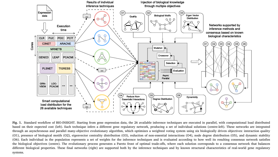
But now, a groundbreaking new tool called BIO-INSIGHT is changing the game. Developed by researchers at the University of Málaga and Catholic University of Valencia, this open-source software leverages a parallel many-objective evolutionary algorithm to produce GRNs that are not only more accurate but also biologically meaningful.
In this article, we’ll explore the 7 revolutionary breakthroughs behind BIO-INSIGHT — and the one costly mistake many researchers still make when inferring gene networks.
What Are Gene Regulatory Networks (GRNs)?
Gene regulatory networks are like the brain of a cell. They determine which genes are activated or silenced in response to environmental cues, developmental signals, or disease states. Understanding GRNs is essential for:
- Identifying disease biomarkers
- Discovering new drug targets
- Advancing personalized medicine
However, inferring these networks from gene expression data is notoriously difficult. Traditional methods often produce conflicting results, even when analyzing the same dataset.
The Problem: Over 26 machine learning techniques exist for GRN inference — but they rarely agree. This inconsistency undermines confidence in their predictions.
The Consensus Crisis in GRN Inference
A 2025 study published in Computers in Biology and Medicine revealed a startling truth: even high-accuracy inference techniques produce vastly different networks. For example, in one test:
- NONLINEARODES predicted a central regulatory hub.
- GENIE3_ET ignored that hub entirely, favoring a decentralized structure.
This lack of consensus isn’t just an academic concern — it leads to false leads in drug discovery and missed biological insights.
💡 Key Insight: Relying on a single inference method is like navigating a maze with one map — you might get somewhere, but it won’t be the optimal path.
Introducing BIO-INSIGHT: The Game-Changer
BIO-INSIGHT (Biologically Informed Optimizer – INtegrating Software to Infer GRNs by Holistic Thinking) is a paradigm shift. Instead of choosing one method, it combines 26 state-of-the-art inference techniques into a unified consensus framework.
But here’s what makes it revolutionary: it doesn’t just average results. It uses a many-objective evolutionary algorithm to optimize for biological plausibility, not just statistical fit.
✅ Key Features:
- Open-source & free (MIT license)
- Built on Java + JMetal framework
- Integrates 26+ inference tools (ARACNE, GENIE3, TIGRESS, etc.)
- Parallel, asynchronous processing for large-scale networks
- Python library available on PyPI:
GENECI
7 Revolutionary Breakthroughs in BIO-INSIGHT
Let’s dive into the 7 game-changing innovations that make BIO-INSIGHT outperform all existing methods.
1. Six Biologically Driven Objectives (Not Just Two)
Most consensus tools optimize for basic network properties like degree distribution. BIO-INSIGHT goes much further, evaluating networks across six biologically grounded objectives:
| OBJECTIVE | BIOLOGICAL RELEVANCE |
|---|---|
| Quality | Promotes high-confidence, coherent interactions |
| Motifs | Favors known regulatory patterns (e.g., feedforward loops) |
| Eigenvector Distribution | Ensures influence follows power-law (hub genes matter) |
| Reduce Non-Essential Interactions | Removes redundant edges via edge betweenness |
| Degree Distribution | Enforces scale-free topology |
| Dynamicity | Tests network stability under ODE simulations |
This multi-faceted approach ensures networks are not just accurate, but biologically realistic.
2. Eigenvector Centrality: The Hidden Influence Metric
While most tools focus on node degree (number of connections), BIO-INSIGHT uses eigenvector centrality to identify genes that are influential because they connect to other influential genes.
This is crucial because in real GRNs, a gene with few connections can still be a master regulator if it controls key hubs.
The eigenvector score for node i is computed as:
$$\text{Ax}=\text{λx}$$where A is the adjacency matrix, x is the eigenvector, and λ is the largest eigenvalue.
BIO-INSIGHT tests whether these scores follow a Pareto (power-law) distribution, a hallmark of biological networks.
3. Dynamic Stability via ODE Modeling
A network might look good on paper — but is it stable? BIO-INSIGHT simulates gene activity over time using a system of nonlinear ordinary differential equations (ODEs):
$$ \frac{d\,y_i}{dt} = f\Bigg(\sum_{j} A_{ji}\,y_j\Bigg) – y_i $$
where:
- yi(t) = expression level of gene i
- Aji = regulatory weight from gene j to i
- f(x) = Hill function modeling nonlinear regulation
The Hill function is defined as:
\[ f(x) = \frac{x^n}{k^n + x^n} \]
with n=2 , k=0.5 — parameters chosen for biological plausibility.
Networks that quickly converge to a stable state score higher, filtering out chaotic or unstable predictions.
4. Edge Betweenness to Eliminate Redundancy
Many inferred networks are overly dense, filled with redundant interactions that obscure true regulatory signals.
BIO-INSIGHT uses edge betweenness centrality to penalize low-impact edges:
$$CB(e) = \sum_{s \neq t} \frac{\sigma_{st}(e)}{\sigma_{st}}$$where σst is the number of shortest paths from s to t , and σst (e) is the number passing through edge e .
Edges with low betweenness are likely redundant. BIO-INSIGHT favors networks where even the weakest edges have high centrality — a sign of functional necessity.
5. Asynchronous Parallel Evolution: Speed Without Sacrifice
With six objectives, the computational cost could be crippling. But BIO-INSIGHT uses an asynchronous, parallel evolutionary model that:
- Allows simultaneous evaluation across generations
- Implements caching to avoid redundant calculations
- Uses adaptive rounding in early evolution stages
- Eliminates intermediate conversions
Result? It handles networks up to 2,000 genes — despite operating in a twice-larger objective space than previous tools.
6. Proven Superiority: +30% Accuracy Gain
BIO-INSIGHT was tested on a benchmark of 106 gene networks from DREAM challenges, SynTReN, GeneNetWeaver, and real databases (BioGRID, RegulonDB).
It was compared against:
- MO-GENECI (previous state-of-the-art)
- Mean, median, weighted mean, Bayesian fusion
- 26 individual inference methods
Results? BIO-INSIGHT dominated in both AUROC and AUPR metrics.
| METHOD | AUPR RANK | AUROC RANK |
|---|---|---|
| BEST_BIO-INSIGHT | 1.52 | 1.70 |
| BEST_MO-GENECI | 2.84 | 2.94 |
| Bayesian Fusion | 5.58 | 5.77 |
Statistical testing (Friedman + Holm) confirmed p-values < 1e-20 — meaning the improvement is overwhelmingly significant.
7. Real-World Clinical Impact: Fibromyalgia & ME/CFS
BIO-INSIGHT isn’t just for academic benchmarks. It was applied to real gene expression data from patients with:
- Myalgic Encephalomyelitis (ME/CFS)
- Fibromyalgia (FM)
- Co-diagnosis (ME/CFS + FM)
The results? It identified condition-specific regulatory interactions with potential biomarker value.
For example:
- CD74–EIF4G2 interaction was uniquely predicted in ME/CFS
- Both genes are involved in immune regulation and protein synthesis
- CD74 is differentially expressed in ME/CFS patients
- Their physical interaction is experimentally confirmed (Affinity Capture-MS)
This proves BIO-INSIGHT can uncover biologically relevant, clinically actionable insights — even in complex, poorly understood diseases.
The 1 Costly Mistake You Must Avoid
Despite these advances, many researchers still make a critical error:
They rely on individual inference methods or simplistic consensus (like averaging) without biological guidance.
Why is this a mistake?
- ❌ Mathematical methods ignore biology — they may produce “accurate” networks that lack functional relevance.
- ❌ No trade-off balancing — conflicting objectives (e.g., stability vs. complexity) go unmanaged.
- ❌ Overfitting to specific datasets — techniques that work on DREAM challenges fail on real data.
BIO-INSIGHT avoids this by optimizing for biological coherence, not just predictive accuracy.
How BIO-INSIGHT Works: Step-by-Step
- Input: Gene expression data (e.g., RNA-seq, microarray)
- Phase 1: Run 26 inference techniques in parallel (Docker containers)
- Phase 2: Feed results into the evolutionary algorithm
- Phase 3: Optimize a weight vector for each technique
- Phase 4: Build consensus network via weighted voting
- Phase 5: Evaluate against 6 biological objectives
- Output: Pareto front of optimal networks
Users can then select the most biologically plausible network using interactive visualizations.
Validation: Does It Really Work?
The study answered 6 key research questions — all with a resounding “yes”:
| RQ | QUESTION | ANSWER |
|---|---|---|
| 1 | Is there enough disparity to justify consensus? | ✅ Yes — networks differ wildly |
| 2 | Do objectives conflict (ensuring trade-offs)? | ✅ Yes — proper evolutionary balance |
| 3 | Do accurate techniques get higher weights? | ❌ No — holistic view wins |
| 4 | Are networks biologically coherent? | ✅ Yes — scale-free, modular, motif-rich |
| 5 | Is biological optimization aligned with accuracy? | ✅ Yes — higher optimization = higher AUPR/AUROC |
| 6 | Is BIO-INSIGHT redundant with individual methods? | ❌ No — it adds novel value |
This rigorous validation confirms BIO-INSIGHT isn’t just another tool — it’s a scientific advancement.
How to Use BIO-INSIGHT (Free & Easy)
You don’t need to be a bioinformatics expert. Here’s how to get started:
# Install via PyPI
pip install GENECI==3.0.1

# Run BIO-INSIGHT
bio-insight run --data expression_data.csv --output results/
Or access the source code on GitHub: 👉 https://github.com/AdrianSeguraOrtiz/BIO-INSIGHT
Includes:
- Docker support
- Interactive visualizations
- Benchmark generators
- Pre-configured datasets
The Future of GRN Inference
BIO-INSIGHT is just the beginning. Future plans include:
- Integration of deep learning models
- Clustering-based optimization to reduce redundancy
- Support for single-cell RNA-seq
- Dynamic encoding beyond simple weight vectors
As the authors note: “The current encoding may be too simplistic for the increasing biological complexity.”
If you’re Interested in Medical Image Segmentation, you may also find this article helpful: 7 Revolutionary Breakthroughs in Thyroid Cancer AI: How DualSwinUnet++ Outperforms Old Models
Final Call to Action
If you’re working on gene network inference, stop relying on outdated, inconsistent methods. The future is biologically guided, multi-objective consensus.
👉 Download BIO-INSIGHT today and see the difference for yourself:
- GitHub: https://github.com/AdrianSeguraOrtiz/BIO-INSIGHT
- PyPI: https://pypi.org/project/GENECI/3.0.1/
- Paper Link: Multifaceted evolution focused on maximal exploitation of domain knowledge for the consensus inference of Gene Regulatory Networks
Join the revolution in systems biology — where accuracy meets biological truth.
Below is the Python code that encapsulates the core logic of the BIO-INSIGHT algorithm, including the asynchronous-like parallel evolutionary process and the six biologically-inspired objective functions.
# BIO-INSIGHT: Biologically Informed Optimizer INtegrating Software to Infer GRNs by Holistic Thinking
# This script is a Python implementation of the model described in the paper:
# "Multifaceted evolution focused on maximal exploitation of domain knowledge for the consensus inference of Gene Regulatory Networks"
# by Adrián Segura-Ortiz, et al. (Computers in Biology and Medicine, 2025)

import numpy as np
import networkx as nx
from scipy.integrate import solve_ivp
from scipy.stats import kstest, powerlaw
import random
import multiprocessing
from functools import lru_cache

# --- Helper Functions & Classes ---

class Individual:
    """Represents an individual in the evolutionary algorithm population."""
    def __init__(self, weights):
        if not np.isclose(np.sum(weights), 1.0):
            raise ValueError("Weights must sum to 1.")
        self.weights = np.array(weights)
        self.fitness = {} # Dictionary to store fitness for each objective

    def __repr__(self):
        return f"Individual(weights={self.weights.round(3)}, fitness={self.fitness})"

def build_consensus_network(individual, confidence_matrices):
    """
    Builds a weighted consensus network from an individual's weights.
    Args:
        individual (Individual): The individual with weights for each technique.
        confidence_matrices (dict): A dictionary where keys are technique names
                                    and values are their confidence matrices (NxN numpy arrays).
    Returns:
        np.ndarray: The resulting weighted adjacency matrix for the consensus network.
    """
    num_genes = list(confidence_matrices.values())[0].shape[0]
    consensus_matrix = np.zeros((num_genes, num_genes))

    for i, tech_name in enumerate(confidence_matrices.keys()):
        consensus_matrix += individual.weights[i] * confidence_matrices[tech_name]

    return consensus_matrix

# --- Objective Functions ---

# Objective 1: Quality
def calculate_quality(consensus_matrix, confidence_matrices):
    """
    Promotes interactions with high confidence from coherent techniques.
    Refactored from the description in the paper.
    Lower is better.
    """
    num_genes = consensus_matrix.shape[0]
    if num_genes == 0: return 1.0

    quality_scores = []

    # Create a stack of confidence matrices for easier vectorized operations
    stacked_matrices = np.stack(list(confidence_matrices.values()), axis=-1)

    for i in range(num_genes):
        for j in range(num_genes):
            if i == j: continue

            confidence_values = stacked_matrices[i, j, :]

            # Penalize discrepancies from the median
            median_conf = np.median(confidence_values)
            distance_penalty = np.mean(np.abs(confidence_values - median_conf))

            # Interaction quality is the consensus confidence penalized by distance
            interaction_quality = consensus_matrix[i, j] * (1 - distance_penalty)
            quality_scores.append(interaction_quality)

    if not quality_scores: return 1.0

    mean_quality = np.mean(quality_scores)
    # The objective is to minimize 1 - mean_quality, which is equivalent to maximizing mean_quality
    return 1.0 - mean_quality

# Objective 2: Motifs
@lru_cache(maxsize=1024) # Cache results for binarized networks
def calculate_motifs(binarized_adj_matrix_tuple):
    """
    Favors networks with a high density of known biological motifs.
    Maximizes the count of predefined motifs.
    Higher is better.
    """
    binarized_adj_matrix = np.array(binarized_adj_matrix_tuple)
    G = nx.from_numpy_array(binarized_adj_matrix, create_using=nx.DiGraph)
    motif_count = 0

    # Simplified motif search for demonstration (e.g., Feed-Forward Loop)
    # A -> B, A -> C, B -> C
    for u in G.nodes():
        successors_u = set(G.successors(u))
        if len(successors_u) < 2: continue
        for v in successors_u:
            for w in successors_u:
                if v == w: continue
                if G.has_edge(v, w):
                    motif_count += 1

    # Normalize by the number of possible triangles to keep the value scaled
    num_nodes = G.number_of_nodes()
    if num_nodes < 3: return 0

    # The paper mentions 4 motifs; this is a simplified example.
    # A more complete implementation would search for all specified motifs.
    normalization_factor = num_nodes * (num_nodes - 1) * (num_nodes - 2)
    return motif_count / normalization_factor if normalization_factor > 0 else 0

# Objective 3: Eigenvector Distribution
@lru_cache(maxsize=1024)
def calculate_eigenvector_distribution(adj_matrix_tuple):
    """
    Evaluates if the gene influence (eigenvector centrality) follows a power-law distribution.
    Uses a goodness-of-fit test for a Pareto (power-law) distribution.
    Higher p-value (closer to 1) is better.
    """
    adj_matrix = np.array(adj_matrix_tuple)
    if np.sum(adj_matrix) == 0: return 0.0

    G = nx.from_numpy_array(adj_matrix, create_using=nx.DiGraph)

    try:
        # Use weight attribute for centrality calculation
        centrality = nx.eigenvector_centrality(G, weight='weight', max_iter=1000, tol=1e-04)
        centrality_values = np.array(list(centrality.values()))

        if len(centrality_values) < 2 or np.all(centrality_values == centrality_values[0]):
            return 0.0

        # Fit to a power-law distribution and perform a Kolmogorov-Smirnov test
        # A positive shift is added to ensure all values are > 0 for the power-law fit
        positive_values = centrality_values[centrality_values > 0]
        if len(positive_values) < 2: return 0.0

        # The paper uses a Pareto test; the powerlaw library provides a good approximation.
        fit = powerlaw.Fit(positive_values, discrete=False, verbose=False)
        return fit.power_law.p
    except (nx.PowerIterationFailedConvergence, nx.NetworkXError):
        return 0.0 # Return a poor score if centrality doesn't converge or graph is problematic

# Objective 4: Reduce Non-Essential Interactions
@lru_cache(maxsize=1024)
def reduce_non_essential_interactions(adj_matrix_tuple):
    """
    Penalizes networks with redundant interactions (low edge betweenness centrality).
    The goal is to maximize the centrality of even the least important edges.
    Higher is better.
    """
    adj_matrix = np.array(adj_matrix_tuple)
    if np.sum(adj_matrix) == 0: return 0.0

    # Invert weights for betweenness calculation, as it expects costs/distances
    G = nx.from_numpy_array(1 - adj_matrix, create_using=nx.DiGraph)

    try:
        # The paper mentions a custom Dijkstra-based implementation for efficiency.
        # Here we use networkx's implementation for simplicity.
        # The 'weight' parameter is crucial for weighted betweenness.
        betweenness = nx.edge_betweenness_centrality(G, weight='weight', normalized=True)
        if not betweenness: return 0.0

        betweenness_values = np.array(list(betweenness.values()))

        # The objective is 1 / weighted_mean of sorted centralities.
        # This is equivalent to maximizing the mean of the least central edges.
        # A simpler proxy is to return the mean value, which we want to maximize.
        return np.mean(betweenness_values)
    except nx.NetworkXError:
        return 0.0

# Objective 5: Degree Distribution
@lru_cache(maxsize=1024)
def calculate_degree_distribution(adj_matrix_tuple):
    """
    Promotes scale-free networks by testing if the degree distribution fits a power-law.
    Higher p-value (closer to 1) is better.
    """
    adj_matrix = np.array(adj_matrix_tuple)
    G = nx.from_numpy_array(adj_matrix, create_using=nx.DiGraph)

    degrees = [d for n, d in G.degree(weight='weight')]
    if len(degrees) < 2 or np.all(degrees == degrees[0]):
        return 0.0

    positive_degrees = [d for d in degrees if d > 0]
    if len(positive_degrees) < 2: return 0.0

    # Use the same power-law fit as in eigenvector distribution
    fit = powerlaw.Fit(positive_degrees, discrete=False, verbose=False)
    return fit.power_law.p

# Objective 6: Dynamicity
def ode_system(t, y, A, n=2, k=0.5):
    """
    System of nonlinear ODEs based on the Hill function to model gene regulation.
    """
    # Hill function for activation
    activation = (y**n) / (k**n + y**n)

    # Regulatory interactions based on the adjacency matrix A
    regulation_term = A.T @ activation

    # Degradation term
    degradation_term = y

    dydt = regulation_term - degradation_term
    return dydt

@lru_cache(maxsize=1024)
def calculate_dynamicity(adj_matrix_tuple):
    """
    Evaluates the dynamic stability of the network. A stable system will converge.
    We measure stability as 1 minus the average deviation from the initial state.
    Higher is better (closer to 1).
    """
    adj_matrix = np.array(adj_matrix_tuple)
    num_genes = adj_matrix.shape[0]
    if num_genes == 0: return 0.0

    # Initial state: all genes expressed at a baseline level
    y0 = np.ones(num_genes)

    # Time span for the simulation
    t_span = [0, 50]

    try:
        # Solve the ODE system
        sol = solve_ivp(
            ode_system,
            t_span,
            y0,
            args=(adj_matrix,),
            method='DOP853', # Similar to Dormand-Prince 5(4)
            dense_output=True
        )

        # Get the final state of the system
        final_state = sol.y[:, -1]

        # Calculate the average deviation from the initial state (1.0)
        # A stable system should not diverge uncontrollably.
        avg_deviation = np.mean(np.abs(final_state - y0))

        # The score is higher for smaller deviations (more stable systems)
        stability_score = 1.0 / (1.0 + avg_deviation)
        return stability_score

    except Exception:
        return 0.0 # Return a poor score if the simulation fails

# --- Evaluation Function ---

def evaluate_individual(individual, confidence_matrices, binarization_threshold=0.5):
    """
    Evaluates an individual against all six objective functions.
    """
    # 1. Build the consensus network
    consensus_matrix = build_consensus_network(individual, confidence_matrices)

    # For caching, convert numpy arrays to tuples of tuples
    consensus_tuple = tuple(map(tuple, consensus_matrix))

    # Binarize for motif calculation
    binarized_matrix = (consensus_matrix > binarization_threshold).astype(int)
    binarized_tuple = tuple(map(tuple, binarized_matrix))

    # 2. Calculate fitness for each objective
    # Note on optimization direction:
    # Quality: Minimize (so we use 1 - score) -> Handled inside function
    # Motifs: Maximize
    # Eigenvector Dist: Maximize
    # Reduce Non-Essential: Maximize
    # Degree Dist: Maximize
    # Dynamicity: Maximize

    fitness = {}
    fitness['quality'] = calculate_quality(consensus_matrix, confidence_matrices)
    fitness['motifs'] = calculate_motifs(binarized_tuple)
    fitness['eigen_dist'] = calculate_eigenvector_distribution(consensus_tuple)
    fitness['reduce_non_essential'] = reduce_non_essential_interactions(consensus_tuple)
    fitness['degree_dist'] = calculate_degree_distribution(consensus_tuple)
    fitness['dynamicity'] = calculate_dynamicity(consensus_tuple)

    individual.fitness = fitness
    return tuple(fitness.values())


# --- Evolutionary Algorithm Components ---

def dominates(ind1, ind2):
    """Checks if individual 1 dominates individual 2."""
    # Assumes all objectives are to be maximized
    better_in_one = False
    for obj in ind1.fitness:
        if ind1.fitness[obj] < ind2.fitness[obj]:
            return False # ind1 is worse in at least one objective
        if ind1.fitness[obj] > ind2.fitness[obj]:
            better_in_one = True
    return better_in_one

def non_dominated_sort(population):
    """Performs non-dominated sorting and returns fronts."""
    fronts = [[]]
    for p in population:
        p.domination_count = 0
        p.dominated_solutions = []
        for q in population:
            if p is q: continue
            if dominates(p, q):
                p.dominated_solutions.append(q)
            elif dominates(q, p):
                p.domination_count += 1
        if p.domination_count == 0:
            fronts[0].append(p)

    i = 0
    while fronts[i]:
        next_front = []
        for p in fronts[i]:
            for q in p.dominated_solutions:
                q.domination_count -= 1
                if q.domination_count == 0:
                    next_front.append(q)
        i += 1
        fronts.append(next_front)

    return fronts[:-1] # Return all non-empty fronts

def crowding_distance(front):
    """Calculates crowding distance for individuals in a front."""
    if not front: return

    num_objectives = len(list(front[0].fitness.values()))
    for ind in front:
        ind.crowding_distance = 0

    for i, obj_key in enumerate(front[0].fitness.keys()):
        front.sort(key=lambda x: x.fitness[obj_key])
        front[0].crowding_distance = float('inf')
        front[-1].crowding_distance = float('inf')

        f_min = front[0].fitness[obj_key]
        f_max = front[-1].fitness[obj_key]

        if f_max == f_min: continue

        for j in range(1, len(front) - 1):
            front[j].crowding_distance += (front[j+1].fitness[obj_key] - front[j-1].fitness[obj_key]) / (f_max - f_min)

def selection(population, k):
    """Selects k individuals using binary tournament selection based on rank and crowding."""
    selected = []
    for _ in range(k):
        p1 = random.choice(population)
        p2 = random.choice(population)

        if p1.rank < p2.rank:
            selected.append(p1)
        elif p2.rank < p1.rank:
            selected.append(p2)
        elif p1.crowding_distance > p2.crowding_distance:
            selected.append(p1)
        else:
            selected.append(p2)
    return selected

def simplex_crossover(p1, p2, eta=2):
    """Simplex Crossover (SPX) for weight vectors that sum to 1."""
    n = len(p1.weights)
    c1_weights = np.zeros(n)
    c2_weights = np.zeros(n)

    # This is a simplified version. A full SPX is more complex.
    # Using a simple blend crossover and re-normalizing for demonstration.
    alpha = random.random()
    c1_weights = alpha * p1.weights + (1 - alpha) * p2.weights
    c2_weights = (1 - alpha) * p1.weights + alpha * p2.weights

    # Ensure weights sum to 1
    c1_weights /= np.sum(c1_weights)
    c2_weights /= np.sum(c2_weights)

    return Individual(c1_weights), Individual(c2_weights)

def polynomial_mutation(individual, eta=20, prob_mut=0.1):
    """Polynomial mutation adapted for simplex."""
    if random.random() > prob_mut:
        return

    weights = individual.weights.copy()
    n = len(weights)

    for i in range(n):
        if random.random() < 1.0 / n:
            delta = 0
            u = random.random()
            if u < 0.5:
                delta = (2 * u)**(1.0 / (eta + 1)) - 1
            else:
                delta = 1 - (2 * (1 - u))**(1.0 / (eta + 1))

            weights[i] += delta

    # Project back to the simplex (ensure non-negative and sum to 1)
    weights[weights < 0] = 0
    if np.sum(weights) > 0:
        weights /= np.sum(weights)
    else: # In case all weights become 0
        weights = np.full(n, 1.0/n)

    individual.weights = weights


# --- Main BIO-INSIGHT Class ---

class BioInsight:
    def __init__(self, inference_techniques, pop_size=100, num_generations=50, num_cores=4):
        self.inference_techniques = inference_techniques
        self.num_techniques = len(inference_techniques)
        self.pop_size = pop_size
        self.num_generations = num_generations
        self.num_cores = num_cores
        self.population = []
        self.confidence_matrices = {}

    def _initialize_population(self):
        """Initializes the population with random weight vectors."""
        self.population = []
        for _ in range(self.pop_size):
            weights = np.random.rand(self.num_techniques)
            weights /= np.sum(weights)
            self.population.append(Individual(weights))

    def _run_inference_techniques(self, expression_data):
        """
        Placeholder for running the 26 inference techniques.
        In a real scenario, this would execute external tools (e.g., in Docker containers).
        Here, we simulate their output with random confidence matrices.
        """
        print("Simulating execution of individual inference techniques...")
        num_genes = expression_data.shape[0]
        for tech in self.inference_techniques:
            # Simulate output: a matrix of confidence scores between 0 and 1
            self.confidence_matrices[tech] = np.random.rand(num_genes, num_genes)
            np.fill_diagonal(self.confidence_matrices[tech], 0) # No self-regulation
        print("Individual inference finished.")

    def run(self, expression_data):
        """Main execution workflow for BIO-INSIGHT."""
        # 1. Get results from individual techniques
        self._run_inference_techniques(expression_data)

        # 2. Initialize population for the evolutionary algorithm
        self._initialize_population()

        # 3. Asynchronous-like parallel evaluation of the initial population
        print("Evaluating initial population...")
        with multiprocessing.Pool(self.num_cores) as pool:
            # Create a list of arguments for the evaluation function
            eval_args = [(ind, self.confidence_matrices) for ind in self.population]
            # Map the function to the arguments
            results = pool.starmap(evaluate_individual, eval_args)

        for i, ind in enumerate(self.population):
            ind.fitness = dict(zip(['quality', 'motifs', 'eigen_dist', 'reduce_non_essential', 'degree_dist', 'dynamicity'], results[i]))

        # 4. Main evolutionary loop (NSGA-II)
        for gen in range(self.num_generations):
            print(f"\n--- Generation {gen + 1}/{self.num_generations} ---")

            # Non-dominated sort and crowding distance
            fronts = non_dominated_sort(self.population)
            for i, front in enumerate(fronts):
                for ind in front:
                    ind.rank = i
                crowding_distance(front)

            # Selection
            parents = selection(self.population, self.pop_size)

            # Crossover and Mutation to create offspring
            offspring = []
            for i in range(0, self.pop_size, 2):
                p1 = parents[i]
                p2 = parents[i+1]
                c1, c2 = simplex_crossover(p1, p2)
                polynomial_mutation(c1)
                polynomial_mutation(c2)
                offspring.extend([c1, c2])

            # Evaluate offspring in parallel
            with multiprocessing.Pool(self.num_cores) as pool:
                eval_args = [(ind, self.confidence_matrices) for ind in offspring]
                results = pool.starmap(evaluate_individual, eval_args)

            for i, ind in enumerate(offspring):
                ind.fitness = dict(zip(['quality', 'motifs', 'eigen_dist', 'reduce_non_essential', 'degree_dist', 'dynamicity'], results[i]))

            # Combine parent and offspring population
            combined_pop = self.population + offspring

            # Select next generation
            fronts = non_dominated_sort(combined_pop)
            next_population = []
            for front in fronts:
                if len(next_population) + len(front) <= self.pop_size:
                    next_population.extend(front)
                else:
                    crowding_distance(front)
                    front.sort(key=lambda x: x.crowding_distance, reverse=True)
                    remaining_space = self.pop_size - len(next_population)
                    next_population.extend(front[:remaining_space])
                    break

            self.population = next_population

            # Log the best fitness from the first front
            best_in_front = max(self.population, key=lambda x: x.fitness['quality'])
            print(f"Sample best fitness (quality): {best_in_front.fitness['quality']:.4f}")

        # 5. Return the final Pareto front
        final_front = non_dominated_sort(self.population)[0]
        print(f"\nEvolution finished. Found {len(final_front)} solutions in the Pareto front.")
        return final_front


if __name__ == '__main__':
    # --- Example Usage ---

    # List of inference techniques (as mentioned in the paper)
    # A subset is used here for brevity.
    TECHNIQUES = [
        "ARACNE", "BC3NET", "C3NET", "CLR", "GENIE3_RF", "GRNBOOST2",
        "MRNET", "PCIT", "TIGRESS", "PLSNET"
    ]

    # Simulate gene expression data (e.g., 50 genes, 100 samples)
    NUM_GENES = 50
    NUM_SAMPLES = 100
    mock_expression_data = np.random.rand(NUM_GENES, NUM_SAMPLES)

    # Instantiate and run BIO-INSIGHT
    bio_insight_model = BioInsight(
        inference_techniques=TECHNIQUES,
        pop_size=50,          # Smaller for quick demo
        num_generations=20,   # Smaller for quick demo
        num_cores=multiprocessing.cpu_count()
    )

    pareto_front_solutions = bio_insight_model.run(mock_expression_data)

    # Display one of the solutions from the Pareto front
    if pareto_front_solutions:
        print("\n--- Example Solution from Pareto Front ---")
        best_solution = pareto_front_solutions[0]
        print(f"Weights: {best_solution.weights.round(3)}")
        print("Fitness values:")
        for obj, val in best_solution.fitness.items():
            print(f"  - {obj}: {val:.4f}")

        # We can now build the final network from this solution
        final_network = build_consensus_network(best_solution, bio_insight_model.confidence_matrices)
        print(f"\nGenerated a {final_network.shape[0]}x{final_network.shape[0]} consensus network matrix.")
Pingback: 7 Breakthrough AI Insights: How Machine Learning Predicts Glioma Grading - aitrendblend.com