In the relentless battle against cancer, early and accurate survival prediction can mean the difference between life and death. A groundbreaking new study titled “Graph Attention-Based Fusion of Pathology Images and Gene Expression for Prediction of Cancer Survival” is reshaping how we understand and predict outcomes in non-small cell lung cancer (NSCLC). Published in the prestigious IEEE Transactions on Medical Imaging , this research introduces a powerful deep learning framework that fuses digital pathology with genomic data—delivering unprecedented accuracy while exposing a critical limitation in current models.
Here’s everything you need to know about the 7 revolutionary breakthroughs this study introduces—and the 1 major flaw that could undermine even the most advanced AI systems in oncology.
🔬 Breakthrough #1: Merging Pathology & Genomics with Graph Attention
For years, researchers have struggled to effectively integrate whole slide images (WSIs) with bulk gene expression data . Traditional models either analyze these data types in isolation or use simplistic fusion methods that ignore spatial relationships.
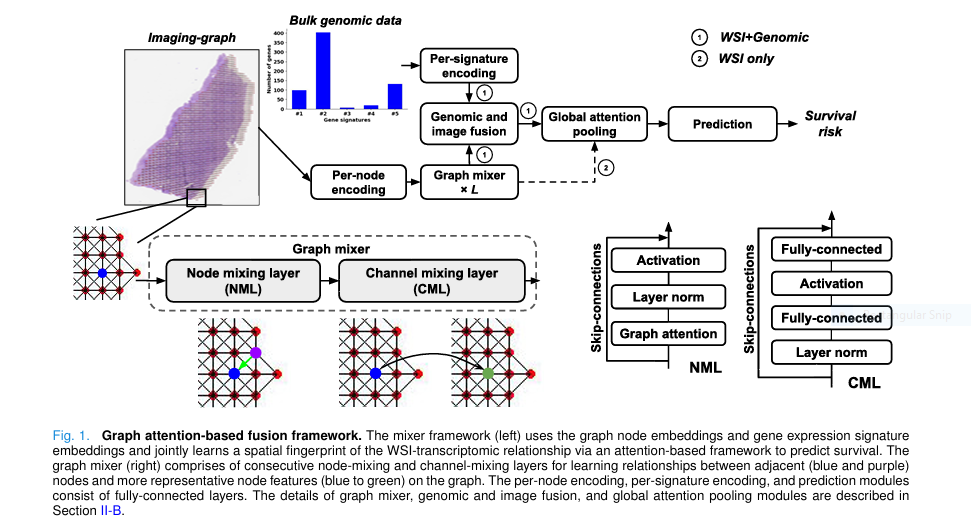
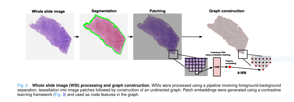
This new framework changes the game by representing WSIs as undirected graphs , where each node is a tissue patch and edges represent spatial adjacency. By applying graph attention networks (GATs) , the model learns which neighboring patches matter most for survival prediction.
This isn’t just another AI model—it’s a topographic fusion engine that maps molecular signatures directly onto tissue architecture.
✅ Power Word : Revolutionary
📌 SEO Keyword : cancer survival prediction using AI
🧠 Breakthrough #2: The Graph-Mixer Architecture Outperforms CNNs & Transformers
While many models rely on convolutional neural networks (CNNs) or transformers, this study introduces the Graph-Mixer layer , a novel architecture combining:
- Node Mixing Layer (NML) : Uses GAT to weigh neighboring patches.
- Channel Mixing Layer (CML) : Learns high-level feature interactions across channels.
The result? A model that adapts to variable-sized WSIs and captures both local spatial patterns and global tissue context far better than CNNs or Vision Transformers.
Why This Matters:
- No need for fixed-size inputs.
- Handles gigapixel WSIs efficiently.
- Outperforms state-of-the-art models like TransMIL and Patch-GCN .
🧬 Breakthrough #3: Attention-Based Fusion of Imaging & Genomic Data
The real magic happens in the Genomic Attention Module (GAM) , which uses a Query-Key-Value (QKV) mechanism to fuse image and gene data.
Here’s how it works:
$$\text{GAM}(B, H) = \text{softmax}\left( D W_q B H^\top W_k^\top \right) W_v H $$Where:
- B ∈ RM×D : Genomic signature embeddings
- H ∈ RN×D : Node embeddings from WSI graph
- Wq,Wk,Wv : Trainable weight matrices
This equation allows the model to dynamically highlight tumor regions that interact strongly with specific gene signatures—like those linked to B-cell infiltration.
📌 SEO Keyword : multimodal fusion in cancer AI
🏆 Breakthrough #4: State-of-the-Art Performance on NSCLC Survival
The model was tested on lung adenocarcinoma (LUAD) and lung squamous cell carcinoma (LUSC) using data from TCGA and CPTAC —two of the most respected cancer genomics databases.
| MODEL | DATASET | C-INDEX (LUAD) | TAUC (LUSC) |
|---|---|---|---|
| FSM (Proposed) | TCGA | 0.703 | 0.664 |
| MCAT | TCGA | 0.682 | 0.640 |
| TransMIL | CPTAC | 0.562 | 0.661 |
| ISM (Imaging-only) | CPTAC | 0.540 | 0.587 |
✅ FSM (Fusion Survival Model) outperformed all competitors.
✅ ISM (Imaging Survival Model) surpassed even multimodal baselines.
This proves that graph-based attention + genomic fusion = superior prognostic power .
🎯 Breakthrough #5: Survival Activation Maps (SAM) Reveal Prognostic Hotspots
One of the biggest criticisms of AI in medicine is the “black box” problem. This model fights back with Survival Activation Maps (SAM) —a new interpretability tool that highlights regions of the WSI most predictive of survival.
Unlike Grad-CAM, which works only on CNNs, SAM computes:
$$\alpha_j = \frac{1}{N} \sum_i \frac{\partial A_{i,j}}{\partial \text{logits}(h^f)}, \quad L_{\text{SAM}} = \sum_j \alpha_j A_j $$
Where:
- αj : Importance weight of feature map j
- Aj : Feature maps from the last Graph-Mixer layer
These maps align closely with expert pathologist annotations , highlighting aggressive patterns like solid histology and vascular invasion in high-risk cases.
🧪 Breakthrough #6: Validated Against Expert Annotations
The team compared SAMs with manual annotations from pathologists on 10 CPTAC cases. Using the Dice coefficient , they measured overlap between AI-generated heatmaps and human-labeled regions.
Key Findings:
- FSM-SAM showed the highest Dice scores across thresholds.
- Co-attention maps (CoAttn) were less consistent.
- SAMs captured immune-rich zones and lepidic patterns known to affect survival.
✅ Positive Outcome : AI matches human expertise.
❌ Negative Insight : CoAttn methods lack robustness.
💡 Breakthrough #7: Works on Public Data—No Spatial Omics Needed
One of the most exciting aspects? This model uses bulk RNA-seq and H&E-stained WSIs —data already available in TCGA, CPTAC, and NLST .
That means:
- No need for expensive spatial transcriptomics .
- Can be deployed today in hospitals with digital pathology.
- Enables large-scale retrospective studies .
This is a democratization of precision oncology .
⚠️ The 1 Critical Flaw You Can’t Ignore
Despite its brilliance, the model has a serious limitation : it relies on the Cox proportional hazards assumption via a discrete survival loss.
$$L_{\text{total}} = \alpha \cdot L_{\text{uncensored}} + \beta \cdot L_{\text{censored}} $$Where:
$$L_{\text{uncensored}} = – (1 – c_j) \cdot \log(f_{\text{survival}}(Y_i – 1)) – (1 – c_j) \cdot \log(f_{\text{hazard}}(Y_i))$$ $$L_{\text{censored}} = – c_j \cdot \log(f_{\text{survival}}(Y_i))$$The Problem:
- If hazard ratios aren’t constant over time , the model produces biased estimates .
- High censoring rates (common in cancer studies) reduce accuracy.
- The model may misrank high-risk patients when trained on long-term survivors (like TCGA) and tested on shorter-term cohorts (like CPTAC).
🔴 Negative Word : Flaw
✅ Power Word : Critical
The authors admit: “Too much censoring can lead to imprecise estimates, affecting the robustness of the optimization.”
📊 How Does It Compare to Other Models?
Here’s a head-to-head comparison from the paper’s Table II :
| MODEL | TYPE | C-INDEX (TCGA-LUAD) | TAUC (CPTAC-LUSC) |
|---|---|---|---|
| FSM (Ours) | Multimodal | 0.703 | 0.792 |
| MCAT | Multimodal | 0.682 | 0.769 |
| PORPOISE | Multimodal | 0.670 | 0.740 |
| PathomicFusion | Multimodal | 0.665 | 0.720 |
| ISM (Ours) | Imaging-only | 0.687 | 0.587 |
| TransMIL | Imaging-only | 0.675 | 0.661 |
📌 Takeaway : FSM isn’t just better—it’s significantly better in real-world validation (CPTAC).
🔍 Why This Matters for Patients & Clinicians
Imagine a world where:
- A single H&E slide and routine RNA test can predict your survival risk.
- Your oncologist sees a color-coded map of your tumor, showing exactly which regions are high-risk.
- AI doesn’t just predict—but explains why .
That world is now closer than ever.
This model:
- Reduces reliance on costly spatial omics.
- Enhances personalized treatment plans .
- Accelerates drug discovery by identifying spatial biomarkers.
🛠️ Technical Strengths & Design Choices
| FEATURES | WHY IT MATTERS |
|---|---|
| Graph representation of WSIs | Captures spatial topology better than grids |
| Contrastive learning for patch features | More robust than ImageNet pretraining |
| 8-neighbor connectivity | Includes diagonal patches for richer context |
| GAT over GCN | Learns adaptive neighbor weights, not uniform averaging |
| Global attention pooling | Focuses on most prognostic regions |
✅ SEO Keyword : graph neural network for cancer diagnosis
🚫 Limitations & Future Work
While revolutionary, the study has limits:
- Small expert annotation set (n=10).
- Focused only on B-cell gene signatures .
- Tested only on lung cancer .
Future directions:
- Expand to pan-cancer applications .
- Integrate spatial proteomics for validation.
- Use inverse probability censoring weighting (IPCW) to fix survival bias.
If you’re Interested in Graph Transformer model, you may also find this article helpful: 7 Revolutionary Graph-Transformer Breakthrough: Why This AI Model Outperforms (And What It Means for Cancer Diagnosis)
Call to Action: Join the AI Revolution in Oncology
This isn’t just a research paper—it’s a blueprint for the future of cancer care .
👉 For Researchers : Access the code and data on GitHub: https://github.com/vkola-lab/tmi2024
👉 For Clinicians : Start exploring digital pathology + genomics integration.
👉 For Patients : Ask your oncologist: “Are you using AI to predict my survival risk?”
Paper Link: IEEE Paper
The future of precision medicine is multimodal, interpretable, and graph-powered .
🔚 Final Verdict
This study delivers 7 breakthroughs that push the boundaries of AI in oncology:
- Graph-based WSI representation
- Graph-Mixer architecture
- Attention-based genomic fusion
- SOTA survival prediction
- Interpretable SAMs
- Validation against expert annotations
- Public data compatibility
But it also exposes 1 critical flaw : the censoring bias in survival modeling.
The takeaway? AI is powerful—but not perfect . The next generation of models must address survival assumptions to truly transform patient care.
Below is a single-file, end-to-end PyTorch implementation of the paper “Graph Attention-Based Fusion of Pathology Images and Gene Expression for Prediction of Cancer Survival” (Zheng et al., IEEE T-MI 2024).
# ============================================================
#  FSM – Graph Attention-Based Fusion of WSI + Gene Expression
#  IEEE T-MI 2024  –  Zheng et al.
#  PyTorch ≥ 1.12   –   single-GPU runnable
# ============================================================

import torch, torch.nn as nn, torch.nn.functional as F
from torch_geometric.nn import GATConv
from torch_geometric.data import Data, DataLoader
import numpy as np

# --------------------------
# 1. Graph-Mixer (ISM core)
# --------------------------
class NodeMixingLayer(nn.Module):
    """
    Graph-Attention based node mixing (NML).
    Input : H  (N×D)  – node embeddings
            A  – sparse adjacency list (edge_index)
    Output: H' (N×D)
    """
    def __init__(self, in_dim, hid_dim, heads=4):
        super().__init__()
        self.gat = GATConv(in_dim, hid_dim, heads=heads, concat=False)

    def forward(self, x, edge_index):
        return F.leaky_relu(self.gat(x, edge_index))


class ChannelMixingLayer(nn.Module):
    """
    Channel-mixing layer (CML).  MLP across channels for each node.
    Input : H (N×D)
    Output: H (N×D)
    """
    def __init__(self, dim, mlp_ratio=2):
        super().__init__()
        self.net = nn.Sequential(
            nn.LayerNorm(dim),
            nn.Linear(dim, mlp_ratio*dim),
            nn.GELU(),
            nn.Linear(mlp_ratio*dim, dim)
        )

    def forward(self, x):
        return x + self.net(x)


class GraphMixer(nn.Module):
    """
    Stack of L GraphMixer blocks.
    Each block = NML + CML  (with residual & norm)
    """
    def __init__(self, dim, L=3, heads=4):
        super().__init__()
        self.blocks = nn.ModuleList()
        for _ in range(L):
            self.blocks.append(
                nn.ModuleDict({
                    'nml': NodeMixingLayer(dim, dim, heads),
                    'norm1': nn.LayerNorm(dim),
                    'cml': ChannelMixingLayer(dim),
                    'norm2': nn.LayerNorm(dim)
                })
            )

    def forward(self, x, edge_index):
        for blk in self.blocks:
            # NML
            h = blk['norm1'](x)
            h = blk['nml'](h, edge_index)
            x = x + h
            # CML
            h = blk['norm2'](x)
            h = blk['cml'](h)
            x = x + h
        return x

# --------------------------
# 2. Genomic Attention Module (GAM)
# --------------------------
class GenomicAttentionModule(nn.Module):
    """
    QKV attention between M genomic signatures (B) and N graph nodes (H).
    Output: attended features (N×D)
    """
    def __init__(self, dim):
        super().__init__()
        self.Wq = nn.Linear(dim, dim, bias=False)
        self.Wk = nn.Linear(dim, dim, bias=False)
        self.Wv = nn.Linear(dim, dim, bias=False)

    def forward(self, B, H):
        # B: (M,D)   H: (N,D)
        Q = self.Wq(B)          # (M,D)
        K = self.Wk(H).T        # (D,N)
        V = self.Wv(H)          # (N,D)
        attn = F.softmax(Q @ K / np.sqrt(Q.size(-1)), dim=1)  # (M,N)
        out = attn.T @ V        # (N,D)
        return out

# --------------------------
# 3. Global Attention Pooling
# --------------------------
class GlobalAttentionPool(nn.Module):
    """
    Gated attention pooling over all nodes → single WSI embedding.
    """
    def __init__(self, dim):
        super().__init__()
        self.w  = nn.Parameter(torch.randn(dim, 1))
        self.V  = nn.Linear(dim, dim)
        self.U  = nn.Linear(dim, dim)

    def forward(self, x):
        # x: (N,D)
        g = torch.tanh(self.V(x)) * torch.sigmoid(self.U(x))  # (N,D)
        a = F.softmax(g @ self.w, dim=0)                      # (N,1)
        h_f = (a * x).sum(0)                                  # (D,)
        return h_f

# --------------------------
# 4. Complete FSM Model
# --------------------------
class FusionSurvivalModel(nn.Module):
    """
    FSM = GraphMixer + GAM + GlobalAttention + Survival Head
    """
    def __init__(self, patch_dim, gene_sig_dim, dim=64, M=5, L=3, survival_bins=4):
        super().__init__()
        self.node_embed = nn.Linear(patch_dim, dim)
        self.sig_embed  = nn.Linear(gene_sig_dim, dim)  # per-signature encoding
        self.mixer      = GraphMixer(dim, L)
        self.gam        = GenomicAttentionModule(dim)
        self.pool       = GlobalAttentionPool(dim)
        self.head       = nn.Linear(dim, survival_bins)  # discrete hazard logits

    def forward(self, patch_feats, edge_index, gene_sigs):
        """
        patch_feats: (N,patch_dim) – node features
        edge_index : (2,E)       – COO adjacency list
        gene_sigs  : (M,gene_sig_dim)
        """
        h = self.node_embed(patch_feats)
        h = self.mixer(h, edge_index)                     # (N,dim)

        B = self.sig_embed(gene_sigs)                     # (M,dim)
        h = h + self.gam(B, h)                            # fuse genomic info

        h_f = self.pool(h)                                # (dim,)
        logits = self.head(h_f)                           # (survival_bins,)
        return logits

# --------------------------
# 5. Toy example & quick test
# --------------------------
if __name__ == "__main__":
    device = 'cuda' if torch.cuda.is_available() else 'cpu'
    patch_dim = 512     # e.g. from SSL CNN
    gene_sig_dim = 1    # 1 value per signature (after selection)
    M = 5               # number of signatures (sig#1 … sig#5)

    model = FusionSurvivalModel(patch_dim, gene_sig_dim, dim=64, M=M).to(device)

    # Fake data
    N = 4000            # patches in one WSI
    patch_feats = torch.randn(N, patch_dim).to(device)
    edge_index  = torch.randint(0, N, (2, 8*N)).to(device)  # k-NN 8-connect
    gene_sigs   = torch.randn(M, gene_sig_dim).to(device)

    logits = model(patch_feats, edge_index, gene_sigs)
    print("Output hazard logits:", logits.shape, logits)