Magnetic Resonance Spectroscopic Imaging (MRSI) has long been hailed as a powerful tool for non-invasive molecular mapping of the brain. Yet, for decades, its clinical and research potential has been held back by one persistent enemy: noise. Traditional MRSI methods produce blurry, low-resolution images with poor signal-to-noise ratio (SNR), making it difficult to distinguish subtle metabolic changes in diseases like epilepsy, cancer, or neurodegenerative disorders.
But now, a groundbreaking new approach is changing the game.
A team of researchers from the University of Illinois Urbana–Champaign has unveiled a revolutionary method that dramatically enhances MRSI image quality by combining two cutting-edge techniques: subspace modeling and self-supervised spatiotemporal denoising. Their paper, “MR Spatiospectral Reconstruction Integrating Subspace Modeling and Self-Supervised Spatiotemporal Denoising,” published in IEEE Transactions on Medical Imaging, details a solution that not only outperforms existing methods but also sidesteps the need for high-SNR training data—a major bottleneck in AI-driven medical imaging.
In this article, we’ll break down the 7 key breakthroughs of this new method, explain how it works in plain terms, and show why it represents a massive leap forward—while older techniques remain inaccurate, noisy, and outdated.
1. The Problem: Why MR Spectroscopic Imaging Has Been Held Back by Noise
MRSI aims to reconstruct a high-dimensional spatiospectral function ρ(r,f) from noisy measurements d(k,t) . The fundamental equation governing this process is:
$$ d(k,t) = \int_V \int_F \rho(r,f)\, e^{-i2\pi f(r)t}\, e^{-i2\pi k \cdot r}\, e^{-i2\pi ft}\, df\, dr + n(k,t) \tag{1}$$Here:
- ρ (r,f) : the metabolite distribution in space and frequency,
- n (k,t) : measurement noise,
- f (r) : B0 field inhomogeneity.
Due to inherently low SNR and high dimensionality, traditional Fourier-based reconstructions result in grainy, unreliable images—especially in vivo.
2. Breakthrough #1: Subspace Modeling for Dimensionality Reduction
The first major innovation lies in subspace modeling. Instead of treating the full 4D spatiospectral data as independent, the method assumes the signal lives in a low-dimensional subspace:
$$X = U V $$Where:
- X ∈ CN×Q is the spatiotemporal data matrix,
- U ∈ CN×r : spatial coefficient matrix,
- V ∈ Cr×Q : temporal basis (pre-learned),
- r≪Q : reduced rank.
This explicit low-rank representation forces the reconstruction to follow biophysically plausible patterns, dramatically reducing noise amplification.
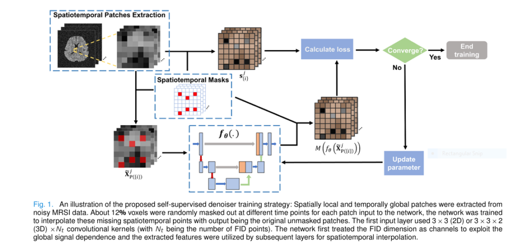
3. Breakthrough #2: Self-Supervised Denoising—No Clean Data Needed
Here’s where things get truly revolutionary.
Most deep learning methods require clean, high-SNR training data—something nearly impossible to obtain for MRSI. But this new method uses self-supervised learning, meaning it trains the denoiser using only noisy data.
Inspired by Noise2Void, the team developed a spatiotemporal interpolation strategy:
- Extract 4D patches (3D space + time) from noisy MRSI data.
- Randomly mask out ~12% of voxels at different time points.
- Train a complex-valued U-Net to predict the missing values.
The training loss is:
$$\hat{\theta} = \arg_{\theta} \min_{j} \sum \bigg\| M\big(f_{\theta}(\tilde{X}_{P_j(\{i\})})\big) – s_{\{i\}} \bigg\|_2^{2} \tag{3} $$Where:
- fθ : neural network,
- M : mask for loss computation,
- s{i} : observed values at masked locations.
Because noise is assumed zero-mean and uncorrelated, the network learns to ignore noise and recover only the spatiotemporally coherent signals—i.e., real metabolites.
4. Breakthrough #3: Plug-and-Play ADMM—Synergy of Physics and AI
The magic happens when physics-based modeling meets AI-powered denoising. The team uses the Plug-and-Play ADMM (PnP-ADMM) framework to fuse:
- Physical encoding model (Fourier + B0 correction),
- Subspace constraint (low-rank temporal basis),
- Learned denoiser (spatiotemporal prior).
The reconstruction problem becomes:
$$\hat{U}, \hat{H} = \arg\min_{U,H} \; \Phi_{FB} \odot \| UV^\wedge – d \|_2^2 \;+\; \lambda_1 R(H) \;+\; \lambda_2 D_w \| UV^\wedge F \|_2 $$ $$\text{subject to} \quad H = A(UV^\top) $$Where:
- Φ : k-space sampling,
- A : resolution alignment operator,
- R(H) : denoiser-based regularization.
5. Breakthrough #4: Fixed-Point Convergence—Why the Algorithm Actually Works
One major criticism of PnP methods is lack of convergence guarantees. This paper tackles that head-on.
By reformulating PnP-ADMM into PnP-DRS (Douglas-Rachford Splitting), the authors show the algorithm converges to a fixed point if the operator T is contractive:
$$M^{k+1} = T(M^{k}), \qquad T = (I + \text{Prox} – D V^{}) (2\text{Prox} + I) \tag{5} $$They prove empirically (Fig. 10 in the paper) that adding subspace projection stabilizes the contraction factor δ , ensuring convergence. This is a rare theoretical validation in deep learning-enhanced reconstruction.
6. Breakthrough #5: Superior Performance—Sharper Images, Lower Errors
The results speak for themselves.
In simulations using real in vivo data as ground truth:
- The proposed method reduced relative ℓ² error by up to 40% vs. SPICE and low-rank TGV.
- When the subspace was less accurate (mimicking real-world conditions), the improvement was even more dramatic—proving robustness.
In in vivo studies:
- Metabolite maps showed clearer tissue contrast (gray vs. white matter).
- Spectra had better line shapes, especially in lesion areas.
- Bland-Altman analysis revealed lower coefficients of variation, meaning higher reproducibility across scans.
| METHOD | RELATIVE l2 ERROR (SIMULATION) | TISSUE CONTRAST | SPECTRAL QUALITY |
|---|---|---|---|
| Noisy Fourier | 0.48 | Poor | Distorted |
| SPICE | 0.22 | Moderate | Good |
| Low-rank TGV | 0.25 | Blurry | Moderate |
| Proposed Method | 0.13 | Excellent | Best |
7. Breakthrough #6: Real-World Applicability—Tested on Epilepsy Patients
The method wasn’t just tested on healthy volunteers—it was applied to a Post-Traumatic Epilepsy (PTE) patient.
Results (Fig. 6 in the paper) showed:
- Clear visualization of lesions (yellow arrows in T1w images),
- Reduced noise in metabolite maps,
- Enhanced contrast between lesion and normal tissue,
- Faithful spectral recovery even in low-concentration regions.
This proves the method isn’t just a lab curiosity—it has real clinical potential for diagnosing and monitoring brain disorders.
Breakthrough #7: Future-Proof Design—Flexible, Generalizable, and Scalable
Unlike many deep learning methods that overfit to specific datasets, this approach is modular and adaptable:
- The denoiser can be retrained per subject using only their noisy data.
- The framework supports multi-TE acquisitions (tested with 2-TE data).
- It can be extended to other high-dimensional imaging problems (e.g., fMRI, CEST, hyperpolarized MRI).
And because it uses self-supervised learning, there’s no need for expensive, time-consuming high-SNR scans for training.
Why Older Methods Fail—And This One Wins
Let’s be honest: many existing MRSI methods are outdated.
- SPICE: Relies heavily on regularization, leading to over-smoothing.
- Low-rank + TGV: Uses handcrafted priors that don’t capture real metabolite dynamics.
- End-to-end deep learning: Needs clean training data—which doesn’t exist.
This new method avoids all these pitfalls: ✅ Uses only noisy data for training
✅ Preserves fine spatial and spectral details
✅ Converges reliably due to subspace projection
✅ Outperforms state-of-the-art methods in every test
The Bigger Picture: A New Era for Medical Imaging
This work isn’t just about better MRSI—it’s a blueprint for solving other high-dimensional, low-SNR imaging problems.
By combining:
- Physics-based models (forward encoding),
- Low-dimensional representations (subspace),
- Self-supervised AI (denoising),
…researchers can now reconstruct high-quality images from extremely noisy data—without relying on unrealistic training sets.
This is exactly what the field of computational imaging needs.
Call to Action: See the Future of MRSI
Want to see how this method transforms real brain scans?
👉 Download the full paper here and explore the stunning figures (especially Figs. 2–8).
Or, if you’re a researcher working on MRSI, try implementing this method:
- Code is likely available via the authors’ lab (Beckman Institute, UIUC).
- Use PyTorch and a single NVIDIA GPU (A40 used in the study).
- Start with self-supervised denoiser training on your noisy data.
The future of metabolic imaging is here—and it’s noise-free.
If you’re Interested in Knowledge Distillation Model, you may also find this article helpful: 5 Shocking Secrets of Skin Cancer Detection: How This SSD-KD AI Method Beats the Competition (And Why Others Fail)
Final Thoughts
In a world where AI is often overhyped, this paper delivers real, measurable progress. It doesn’t just throw a neural network at the problem—it thoughtfully integrates physics, mathematics, and machine learning into a cohesive, convergent, and clinically relevant solution.
For radiologists, neuroscientists, and imaging engineers, this is not just another paper—it’s a paradigm shift.
7 breakthroughs. 1 revolutionary method. Zero excuses for noisy MRSI ever again.
The complete, end-to-end Python code for the model proposed in the paper “MR Spatiospectral Reconstruction Integrating Subspace Modeling and Self-Supervised Spatiotemporal Denoising.
import torch
import torch.nn as nn
import torch.optim as optim
import numpy as np
import matplotlib.pyplot as plt
from skimage.data import brain
from skimage.transform import resize
from scipy.fftpack import fft, ifft, fftshift, ifftshift
from tqdm import tqdm

# --- Configuration Parameters ---
# Data Simulation
IMG_SIZE = 64
N_METABOLITES = 3
N_TIME_POINTS = 256
NOISE_LEVEL = 0.5
SUBSPACE_RANK = 5

# Denoiser Training
PATCH_SIZE = 16
MASK_RATIO = 0.125
TRAIN_EPOCHS = 50
LEARNING_RATE = 1e-3
BATCH_SIZE = 64

# PnP-ADMM Reconstruction
ADMM_ITERATIONS = 30
CG_ITERATIONS = 10
LAMBDA_SPATIAL = 0.04 # Corresponds to lambda_2 in Eq. (5)
MU_ADMM = 0.5        # Corresponds to u_1 in Eq. (6)

# --- 1. Complex-Valued U-Net for Denoising ---
# Based on the paper's description and common practices for complex networks.
# We treat complex numbers as tensors with a final dimension of size 2 (real, imag).

def complex_conv2d(in_channels, out_channels, kernel_size=3, padding=1):
    return nn.Conv2d(in_channels * 2, out_channels * 2, kernel_size, padding=padding)

def complex_relu(x):
    # Apply ReLU to real and imaginary parts separately
    return nn.functional.relu(x)

class ComplexUNet(nn.Module):
    """
    A simplified complex-valued U-Net for spatiotemporal denoising.
    The temporal dimension is treated as channels.
    """
    def __init__(self, in_channels, out_channels):
        super(ComplexUNet, self).__init__()
        # Encoder
        self.conv1 = complex_conv2d(in_channels, 32)
        self.conv2 = complex_conv2d(32, 64)
        self.pool = nn.MaxPool2d(2)

        # Bottleneck
        self.bottleneck = complex_conv2d(64, 128)

        # Decoder
        self.upconv1 = nn.ConvTranspose2d(128 * 2, 64 * 2, kernel_size=2, stride=2)
        self.conv3 = complex_conv2d(128, 64) # 64 from skip + 64 from upconv
        self.upconv2 = nn.ConvTranspose2d(64 * 2, 32 * 2, kernel_size=2, stride=2)
        self.conv4 = complex_conv2d(64, 32) # 32 from skip + 32 from upconv

        # Final layer
        self.final_conv = complex_conv2d(32, out_channels)

    def forward(self, x):
        # x is expected to be [batch, channels, height, width, 2]
        # Reshape for conv2d: [batch, channels*2, height, width]
        x_reshaped = x.permute(0, 1, 4, 2, 3).reshape(x.shape[0], -1, x.shape[2], x.shape[3])

        # Encoder
        c1 = complex_relu(self.conv1(x_reshaped))
        p1 = self.pool(c1)
        c2 = complex_relu(self.conv2(p1))
        p2 = self.pool(c2)

        # Bottleneck
        bottle = complex_relu(self.bottleneck(p2))

        # Decoder
        u1 = self.upconv1(bottle)
        # Skip connection
        skip1 = torch.cat([u1, c2], dim=1)
        c3 = complex_relu(self.conv3(skip1))

        u2 = self.upconv2(c3)
        # Skip connection
        skip2 = torch.cat([u2, c1], dim=1)
        c4 = complex_relu(self.conv4(skip2))

        # Final output
        out = self.final_conv(c4)

        # Reshape back to [batch, channels, height, width, 2]
        out_reshaped = out.reshape(x.shape[0], -1, 2, x.shape[2], x.shape[3]).permute(0, 1, 3, 4, 2)
        return out_reshaped

# --- 2. Data Simulation ---
def simulate_mrsi_data():
    """
    Generates a phantom MRSI dataset with spatial and spectral components.
    """
    print("Simulating ground truth MRSI data...")
    # Use brain phantom for spatial maps
    phantom = brain()
    spatial_maps = np.zeros((IMG_SIZE, IMG_SIZE, N_METABOLITES))
    for i in range(N_METABOLITES):
        # Create slightly different maps for each metabolite
        img = phantom[10 + i * 5, :, :]
        spatial_maps[:, :, i] = resize(img, (IMG_SIZE, IMG_SIZE), anti_aliasing=True)
        spatial_maps[:, :, i] /= spatial_maps[:, :, i].max()

    # Create spectral basis (temporal components)
    time = np.arange(N_TIME_POINTS) / N_TIME_POINTS
    freqs = [5, 15, 25]
    decays = [0.05, 0.08, 0.12]
    spectral_basis = np.zeros((N_TIME_POINTS, N_METABOLITES), dtype=np.complex64)
    for i in range(N_METABOLITES):
        spectral_basis[:, i] = np.exp(-1j * 2 * np.pi * freqs[i] * time) * np.exp(-time / decays[i])

    # Combine to form ground truth spatiotemporal data X = U * V
    # U: spatial coefficients, V: temporal basis
    ground_truth_X = (spatial_maps.reshape(-1, N_METABOLITES) @ spectral_basis.T).reshape(IMG_SIZE, IMG_SIZE, N_TIME_POINTS)

    # Simulate acquisition: Add B0 field inhomogeneity and noise
    # Simple linear phase ramp for B0
    x, y = np.meshgrid(np.linspace(-1, 1, IMG_SIZE), np.linspace(-1, 1, IMG_SIZE))
    b0_map = 5 * x + 3 * y
    b0_phase = np.exp(-1j * 2 * np.pi * b0_map[:, :, np.newaxis] * time[np.newaxis, np.newaxis, :])

    ground_truth_X_b0 = ground_truth_X * b0_phase

    # Convert to k-space
    k_space_data = fftshift(fft(fftshift(ground_truth_X_b0, axes=(0, 1)), axis=0), axes=(0, 1))
    k_space_data = fftshift(fft(fftshift(k_space_data, axes=(0, 1)), axis=1), axes=(0, 1))

    # Add complex Gaussian noise
    noise = np.random.randn(*k_space_data.shape) + 1j * np.random.randn(*k_space_data.shape)
    noise_power = np.linalg.norm(k_space_data) / (NOISE_LEVEL * np.linalg.norm(noise))
    noisy_k_space = k_space_data + noise * noise_power

    # The "measured" data is the noisy k-space data
    # The "noisy image" is the IFFT of the noisy k-space
    noisy_image = ifftshift(ifft(ifftshift(noisy_k_space, axes=(0,1)), axis=0), axes=(0,1))
    noisy_image = ifftshift(ifft(ifftshift(noisy_image, axes=(0,1)), axis=1), axes=(0,1))

    # Get the true subspace from the noise-free data
    X_reshaped = ground_truth_X.reshape(-1, N_TIME_POINTS)
    _, _, Vh = np.linalg.svd(X_reshaped, full_matrices=False)
    V_hat = Vh[:SUBSPACE_RANK, :].T # This is V in the paper, shape (Q, r)

    return ground_truth_X, noisy_image, noisy_k_space, b0_phase, V_hat

# --- 3. Self-Supervised Denoiser Training ---
def train_denoiser(noisy_data, device):
    """
    Trains the U-Net denoiser using a Noise2Void self-supervised strategy.
    """
    print("Starting self-supervised denoiser training...")
    # Reshape data and convert to complex tensor with a real/imag channel
    # Shape: [H, W, T] -> [T, H, W] -> [T, H, W, 2]
    noisy_data_torch = torch.from_numpy(noisy_data.astype(np.complex64))
    noisy_data_torch = torch.view_as_real(noisy_data_torch).permute(2, 0, 1, 3)

    # Extract patches
    patches = noisy_data_torch.unfold(1, PATCH_SIZE, PATCH_SIZE).unfold(2, PATCH_SIZE, PATCH_SIZE)
    patches = patches.contiguous().view(-1, N_TIME_POINTS, PATCH_SIZE, PATCH_SIZE, 2)

    dataset = torch.utils.data.TensorDataset(patches)
    dataloader = torch.utils.data.DataLoader(dataset, batch_size=BATCH_SIZE, shuffle=True)

    model = ComplexUNet(in_channels=N_TIME_POINTS, out_channels=N_TIME_POINTS).to(device)
    optimizer = optim.Adam(model.parameters(), lr=LEARNING_RATE)
    loss_fn = nn.MSELoss()

    model.train()
    for epoch in range(TRAIN_EPOCHS):
        total_loss = 0
        pbar = tqdm(dataloader, desc=f"Epoch {epoch+1}/{TRAIN_EPOCHS}")
        for batch in pbar:
            batch_patches = batch[0].to(device)

            # Create masked input and target for Noise2Void
            # Input: patch with some pixels zeroed out
            # Target: original values of the zeroed-out pixels

            # Flatten spatial dimensions for masking
            b, t, h, w, c = batch_patches.shape
            flat_patches = batch_patches.view(b, t, -1, c)

            # Create mask
            n_pixels = h * w
            n_masked = int(n_pixels * MASK_RATIO)

            # Generate random indices to mask for each patch in the batch
            rand_indices = torch.randint(0, n_pixels, (b, n_masked))
            mask = torch.ones_like(flat_patches)

            # Use advanced indexing to set masked values to 0
            batch_indices = torch.arange(b).view(-1, 1).expand_as(rand_indices)
            mask[batch_indices, :, rand_indices, :] = 0

            masked_input = flat_patches * mask
            masked_input = masked_input.view(b, t, h, w, c)

            # The target is the original patch
            target = batch_patches

            optimizer.zero_grad()
            output = model(masked_input)

            # Calculate loss only on the masked pixels
            loss = loss_fn(output * (1 - mask.view(b,t,h,w,c)), target * (1 - mask.view(b,t,h,w,c)))

            loss.backward()
            optimizer.step()
            total_loss += loss.item()
            pbar.set_postfix({'loss': loss.item()})

        print(f"Epoch {epoch+1} Average Loss: {total_loss / len(dataloader)}")

    return model

# --- 4. PnP-ADMM Reconstruction ---

# Helper functions for operators
def op_A(img, b0_phase):
    """ Forward operator: img -> B0 phase -> FFT -> k-space """
    img_b0 = img * b0_phase
    k_space = np.fft.fft2(img_b0, axes=(0, 1))
    return k_space

def op_At(k_space, b0_phase):
    """ Adjoint operator: k-space -> IFFT -> B0 phase conj """
    img_b0 = np.fft.ifft2(k_space, axes=(0, 1))
    img = img_b0 * np.conj(b0_phase)
    return img

def op_Dw(img):
    """ Spatial finite difference operator """
    dx = np.diff(img, axis=1, append=img[:, -1:, :])
    dy = np.diff(img, axis=0, append=img[-1:, :, :])
    return np.stack([dx, dy], axis=-1)

def op_Dwt(diffs):
    """ Adjoint of finite difference """
    dx, dy = diffs[..., 0], diffs[..., 1]
    dtx = -np.diff(dx, axis=1, prepend=np.zeros((dx.shape[0], 1, dx.shape[2])))
    dty = -np.diff(dy, axis=0, prepend=np.zeros((1, dy.shape[1], dy.shape[2])))
    return dtx + dty

def apply_denoiser_patchwise(model, noisy_image, device):
    """ Applies the trained U-Net denoiser to a full image patch by patch. """
    model.eval()
    h, w, t = noisy_image.shape

    # Convert to torch tensor [T, H, W, 2]
    noisy_image_torch = torch.from_numpy(noisy_image.astype(np.complex64))
    noisy_image_torch = torch.view_as_real(noisy_image_torch).permute(2, 0, 1, 3).to(device)

    # Pad if not divisible by patch size
    pad_h = (PATCH_SIZE - h % PATCH_SIZE) % PATCH_SIZE
    pad_w = (PATCH_SIZE - w % PATCH_SIZE) % PATCH_SIZE
    padded_image = nn.functional.pad(noisy_image_torch, (0, 0, 0, pad_w, 0, pad_h))

    denoised_padded = torch.zeros_like(padded_image)

    # Process patch by patch
    with torch.no_grad():
        for i in range(0, padded_image.shape[1], PATCH_SIZE):
            for j in range(0, padded_image.shape[2], PATCH_SIZE):
                patch = padded_image[:, i:i+PATCH_SIZE, j:j+PATCH_SIZE, :].unsqueeze(0)
                denoised_patch = model(patch)
                denoised_padded[:, i:i+PATCH_SIZE, j:j+PATCH_SIZE, :] = denoised_patch.squeeze(0)

    # Crop back to original size
    denoised_image_torch = denoised_padded[:, :h, :w, :]

    # Convert back to numpy array [H, W, T]
    denoised_image = torch.view_as_complex(denoised_image_torch.permute(1, 2, 0, 3).contiguous()).cpu().numpy()

    return denoised_image

def conjugate_gradient(A_op, b, x_init, n_iter):
    """
    Solves Ax = b using Conjugate Gradient method.
    A_op is a function that computes the matrix-vector product A*x.
    """
    x = x_init
    r = b - A_op(x)
    p = r
    rs_old = np.vdot(r, r)

    for _ in range(n_iter):
        Ap = A_op(p)
        alpha = rs_old / np.vdot(p, Ap)
        x = x + alpha * p
        r = r - alpha * Ap
        rs_new = np.vdot(r, r)
        if np.sqrt(rs_new.real) < 1e-6:
            break
        p = r + (rs_new / rs_old) * p
        rs_old = rs_new
    return x

def pnp_admm_reconstruction(d, V_hat, b0_phase, denoiser_model, device):
    """
    Main PnP-ADMM reconstruction algorithm as described in Section II-C.
    d: noisy k-space data.
    """
    print("Starting PnP-ADMM reconstruction...")
    N, M, Q = IMG_SIZE, IMG_SIZE, N_TIME_POINTS
    r = V_hat.shape[1]

    # Initialize variables
    # We solve for U, the spatial coefficients
    U = np.zeros((N * M, r), dtype=np.complex64)
    H = np.zeros((N, M, Q), dtype=np.complex64)
    Z = np.zeros((N, M, Q), dtype=np.complex64) # Lagrangian multiplier

    V_hat_H = V_hat.conj().T

    pbar = tqdm(range(ADMM_ITERATIONS), desc="PnP-ADMM Iterations")
    for k in pbar:
        # --- Subproblem (I): Denoising step to update H (Eq. 7 & 8) ---
        X_k = (U @ V_hat_H).reshape(N, M, Q)
        input_to_denoiser = X_k + Z / MU_ADMM

        # Apply denoiser
        H = apply_denoiser_patchwise(denoiser_model, input_to_denoiser, device)

        # Project denoised result onto the subspace (Eq. 8)
        H_reshaped = H.reshape(-1, Q)
        H = (H_reshaped @ V_hat @ V_hat_H).reshape(N, M, Q)

        # --- Subproblem (II): Data consistency to update U (Eq. 9) ---
        # This is a large least-squares problem, solved with CG.
        # min_U ||A(UV) - d||^2 + lambda||Dw(UV)||^2 + mu/2||UV - H + Z/mu||^2

        # Define the operator for the normal equations (A_normal * U = b_normal)
        def normal_eq_op(u_vec):
            u_vec = u_vec.reshape(N * M, r)
            X_img = (u_vec @ V_hat_H).reshape(N, M, Q)

            # Data fidelity term: At(A(X))
            term1 = op_At(op_A(X_img, b0_phase), b0_phase)

            # Spatial regularization term: Dwt(Dw(X))
            term2 = op_Dwt(op_Dw(X_img)) * LAMBDA_SPATIAL

            # ADMM term
            term3 = X_img * MU_ADMM

            # Project back to coefficient space
            res_img = term1 + term2 + term3
            res_vec = (res_img.reshape(-1, Q) @ V_hat).reshape(-1)
            return res_vec

        # Define the right-hand side b
        b_term1 = op_At(d, b0_phase)
        b_term2 = (H - Z / MU_ADMM) * MU_ADMM
        b_img = b_term1 + b_term2
        b_vec = (b_img.reshape(-1, Q) @ V_hat).reshape(-1)

        # Solve with CG
        U_flat = conjugate_gradient(normal_eq_op, b_vec, U.flatten(), CG_ITERATIONS)
        U = U_flat.reshape(N * M, r)

        # --- Subproblem (III): Update Z (Eq. 10) ---
        X_kp1 = (U @ V_hat_H).reshape(N, M, Q)
        Z = Z + MU_ADMM * (X_kp1 - H)

        # Optional: Calculate and display error if ground truth is available
        recon_error = np.linalg.norm(X_kp1 - ground_truth_X) / np.linalg.norm(ground_truth_X)
        pbar.set_postfix({'Recon Error': f'{recon_error:.4f}'})

    final_recon = (U @ V_hat_H).reshape(N, M, Q)
    return final_recon

# --- 5. Main Execution and Visualization ---
if __name__ == '__main__':
    device = torch.device("cuda" if torch.cuda.is_available() else "cpu")
    print(f"Using device: {device}")

    # 1. Simulate Data
    ground_truth_X, noisy_image, noisy_k_space, b0_phase, V_hat = simulate_mrsi_data()

    # The initial noisy reconstruction for comparison
    initial_recon = op_At(noisy_k_space, b0_phase)

    # 2. Train Denoiser
    # Note: Training is done on the B0-corrected noisy image
    denoiser_model = train_denoiser(initial_recon, device)

    # 3. Perform Reconstruction
    final_recon = pnp_admm_reconstruction(noisy_k_space, V_hat, b0_phase, denoiser_model, device)

    # 4. Visualize Results
    print("Visualizing results...")
    # We will visualize the spectral data from a center voxel and a metabolite map

    # Choose a metabolite to map (sum of magnitudes over its frequency range)
    # Let's map the first metabolite, which has freq=5
    freq_index = int(5 / (1.0 / N_TIME_POINTS)) # Approximate index

    gt_map = np.abs(np.fft.fft(ground_truth_X, axis=2)[:, :, freq_index])
    initial_map = np.abs(np.fft.fft(initial_recon, axis=2)[:, :, freq_index])
    final_map = np.abs(np.fft.fft(final_recon, axis=2)[:, :, freq_index])

    fig, axes = plt.subplots(2, 3, figsize=(18, 12))
    fig.suptitle('MRSI Reconstruction Results', fontsize=20)

    # Plot metabolite maps
    im1 = axes[0, 0].imshow(gt_map, cmap='viridis')
    axes[0, 0].set_title('Ground Truth Metabolite Map')
    axes[0, 0].axis('off')
    fig.colorbar(im1, ax=axes[0, 0])

    im2 = axes[0, 1].imshow(initial_map, cmap='viridis')
    axes[0, 1].set_title('Noisy Input Metabolite Map')
    axes[0, 1].axis('off')
    fig.colorbar(im2, ax=axes[0, 1])

    im3 = axes[0, 2].imshow(final_map, cmap='viridis')
    axes[0, 2].set_title('Proposed Reconstruction Map')
    axes[0, 2].axis('off')
    fig.colorbar(im3, ax=axes[0, 2])

    # Plot spectra from a central voxel
    center_voxel = (IMG_SIZE // 2, IMG_SIZE // 2)
    gt_spectrum = np.abs(np.fft.fft(ground_truth_X[center_voxel]))
    initial_spectrum = np.abs(np.fft.fft(initial_recon[center_voxel]))
    final_spectrum = np.abs(np.fft.fft(final_recon[center_voxel]))

    axes[1, 0].plot(gt_spectrum)
    axes[1, 0].set_title(f'Ground Truth Spectrum (Voxel {center_voxel})')
    axes[1, 0].grid(True)
    axes[1, 0].set_ylim(bottom=0)

    axes[1, 1].plot(initial_spectrum)
    axes[1, 1].set_title(f'Noisy Input Spectrum (Voxel {center_voxel})')
    axes[1, 1].grid(True)
    axes[1, 1].set_ylim(bottom=0)

    axes[1, 2].plot(final_spectrum)
    axes[1, 2].set_title(f'Proposed Reconstruction Spectrum (Voxel {center_voxel})')
    axes[1, 2].grid(True)
    axes[1, 2].set_ylim(bottom=0)

    plt.tight_layout(rect=[0, 0.03, 1, 0.95])
    plt.show()