Skin cancer is one of the most common—and most deadly—forms of cancer worldwide. If detected at an advanced stage, melanoma, the most fatal type, has a 10-year survival rate of less than 39%. But here’s the hopeful news: early detection can boost that survival rate to over 93%. The challenge? Accurate, timely diagnosis. Dermatologists, even the most skilled, face a complex, subjective task when analyzing skin lesions. This is where artificial intelligence (AI) steps in, not to replace doctors, but to empower them with a powerful, objective tool.
A groundbreaking new study from Atatürk University, published in Engineering Applications of Artificial Intelligence, has unveiled a revolutionary AI framework that achieves an astonishing 83.04% average accuracy in multi-label skin lesion classification. This isn’t just an incremental improvement; it’s a 2.14% leap over the current state-of-the-art, setting a new benchmark for what’s possible in computer-aided diagnosis (CAD).
In this article, we’ll dive deep into the 7 key breakthroughs of this novel AI model, explain why older methods are falling short, and explore how this technology is poised to transform dermatology. Whether you’re a medical professional, a tech enthusiast, or someone concerned about skin health, this is the future of cancer detection.
The Critical Flaw in Traditional Skin Cancer Detection
Before we explore the solution, let’s understand the problem. Dermatologists traditionally rely on rule-based systems like the Seven-Point Checklist (SPC). This method assesses a lesion based on seven criteria—such as the presence of a black/whitish veil, irregular streaks, or atypical pigment networks—assigning points to determine if it’s likely melanoma.
While invaluable, this process has significant drawbacks:
- High Subjectivity: Two experts can interpret the same image differently.
- Information Overload: Evaluating multiple labels (e.g., “Pigment Network: Atypical,” “Vascular Structures: Present”) simultaneously is cognitively taxing.
- Data Silos: Doctors often look at clinical photos (showing the big picture) and dermoscopy images (a magnified view of the skin’s surface) separately, potentially missing crucial connections.
Older AI models have tried to help, but they’ve been limited. Many use only a single type of image (either clinical or dermoscopy), which doesn’t reflect real-world practice. Others attempt to combine data but do so in a simplistic way, like simple averaging, failing to capture the deep, complex relationships between different data sources.
Breakthrough #1: A Multi-Modal Approach That Mirrors Real-World Diagnosis
The most significant leap in this new AI model is its multi-modal design. It doesn’t just look at one image; it intelligently integrates three distinct data streams:
- Dermoscopy Images: High-magnification views revealing subsurface structures.
- Clinical Images: Standard photos showing the lesion’s context on the body.
- Patient Meta-Data: Information like age and sex, which can be crucial for diagnosis.
This mirrors how a dermatologist works, combining visual evidence with patient history. The study’s results are clear: using all three modalities together (DCIHMM) achieves an 83.04% accuracy, significantly outperforming models that use only dermoscopy images (79.72%) or only clinical images (70.57%).
| MODALITY | AVERAGE ACCURACY (%) | IMPROVEMENT OVER SINGLE-MODALITY |
|---|---|---|
| Clinical Image (CIM) | 70.57 | – |
| Dermoscopy Image (DIM) | 79.72 | +13% vs. CIM |
| Hybrid Meta-Modality (DCIHMM) | 83.04 | +4.2% vs. DIM |
Table 1: Accuracy comparison showing the power of multi-modal fusion.
Breakthrough #2: A Hybrid Fusion Strategy for Maximum Information Transfer
It’s not enough to just have multiple data sources; you need a smart way to combine them. This model uses a hybrid fusion strategy, which is far more sophisticated than simple averaging.
Here’s how it works:
- Two separate “branches” of the AI network first analyze the dermoscopy and clinical images independently, extracting their unique features.
- These features are then concatenated (joined together) into a single, richer data stream.
- This combined stream is fed into a third “hybrid-meta” branch, where it is fused with the patient’s meta-data.
This step-by-step, hybrid approach allows the AI to learn complex interactions between the visual data and the patient’s background, creating a far more comprehensive diagnostic picture than any single method could achieve.
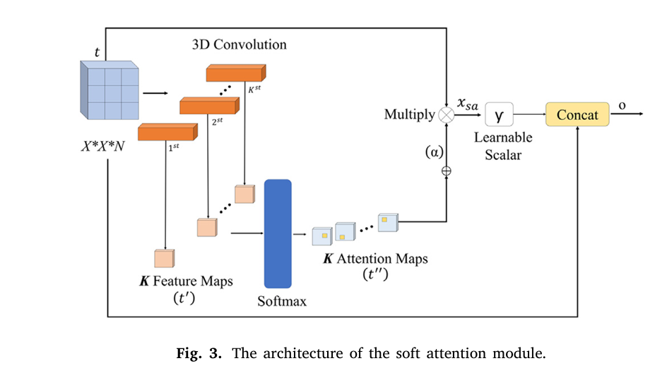
Breakthrough #3: Soft Attention Mechanism – Teaching the AI Where to Look
One of the biggest challenges in medical imaging is that only a small part of an image is actually relevant. Hair, veins, and other artifacts can clutter the view. This model solves this with a soft attention module.
Think of it as a spotlight. The AI learns to assign high “weights” to the pixels that are most important for diagnosing the lesion, effectively dimming the irrelevant background noise. This allows the network to focus its computational power on the discriminative parts of the skin lesion.
The impact is dramatic. When the researchers compared the model with and without the soft attention module, the results were undeniable.
| MODEL VERSION | AVERAGE ACCURACY (%) | IMPROVEMENT |
|---|---|---|
| Without Soft Attention | 79.68 | – |
| With Soft Attention | 83.04 | +4.2% |
Table 2: The transformative effect of the soft attention module.
The attention module works by generating a set of attention maps. These maps are normalized using a softmax function and then used to scale the original feature values. The final output is a combination of the original features and the attentively scaled features, creating a powerful, focused representation.
The mathematical formulation is as follows. A feature tensor t∈Rh×w×d is processed through 3D convolutions to create an intermediate map t′ , which is then normalized:
$$t” = \text{softmax}(t’) = \frac{\exp(t’_{ij})}{\sum_{i=1}^{w} \sum_{j=1}^{h} \exp(t’_{ij})} $$The attention maps are aggregated into a unified map α :
$$\alpha = \sum_{k=1}^{K} \text{softmax}(t’) $$This map is then used to scale the features (xsa=γtα ), and the final output o is produced by adding this scaled feature back to the original, creating a residual connection:
$$o = t + x_{sa} $$
Breakthrough #4: A Modified Xception Backbone for Efficient, Powerful Feature Extraction
The foundation of the AI’s vision is built on a modified Xception architecture. Xception is a powerful deep learning model known for its efficiency and accuracy, using “depthwise separable convolutions” to reduce computational cost.
The researchers made key modifications to tailor it for this specific task:
- They reduced the number of layers in the middle flow from 24 to just 3. This prevents overfitting on the relatively small medical dataset.
- They removed two layers from the exit flow, streamlining the process.
This modified backbone is used in the first two branches of the network, ensuring that both the clinical and dermoscopy images are analyzed with a powerful, yet efficient, engine.
Breakthrough #5: Late Fusion for Robust, Probability-Based Decision Making
After the three branches have processed their respective data, the model needs to make a final decision. It uses a late fusion scheme, which means it combines the predictions at the very end.
Instead of just taking a majority vote (which discards valuable probability information), this model uses an average late fusion approach. It takes the prediction probabilities from all three branches and averages them. The final diagnosis is the label with the highest average probability.
This is mathematically represented as:
$$P_k = \frac{1}{3} \sum_{m=1}^{3} P_{m,k}$$
where Pk is the final averaged probability for label k , and Pm,k is the prediction probability from the mth branch (dermoscopy, clinical, or hybrid-meta).
This method is more robust and utilizes the full confidence information from each branch.
Breakthrough #6: State-of-the-Art Performance on a Real-World Dataset
The true test of any AI model is its performance on real, publicly available data. This model was evaluated on the Seven-Point Criteria Evaluation (SPC) dataset, a well-established benchmark with 1,011 patient cases.
The results were exceptional. As shown in the table below, the proposed model achieved the highest average accuracy of 83.04%, outperforming all other state-of-the-art methods.
| METHOD | AVERAGE ACCURACY (%) |
|---|---|
| Alzahrani et al. (2019) | 66.7 |
| EmbeddingNet (Yap et al., 2018) | 71.7 |
| TripleNet (Ge et al., 2017) | 72.7 |
| Kawahara et al. (2018) | 73.7 |
| FusionM4Net-SS (Tang et al., 2022) | 77.0 |
| CC (Wang et al., 2021a) | 81.3 |
| Proposed Model | 83.04 |
Table 3: Comparison with state-of-the-art methods on the SPC dataset.
It didn’t just win on average; it achieved the highest accuracy for nearly every individual checklist criterion, including the final diagnosis label.
Breakthrough #7: Superior Performance Even on Imbalanced Data
A major challenge in medical datasets is class imbalance—some conditions (like Nevus) are far more common than others (like Basal Cell Carcinoma). Many AI models struggle with this, becoming biased toward the more frequent classes.
The proposed model, however, demonstrated consistent and high performance across all labels, even without using data balancing techniques. This robustness is a critical advantage, proving its potential for real-world clinical use where data imbalance is the norm, not the exception.
Why This Matters: A Future of Faster, More Accurate Diagnoses
This AI model is more than just a research project. It represents a paradigm shift in dermatology. By combining multi-modal data, a hybrid fusion strategy, and a soft attention mechanism, it creates a diagnostic tool that is not only more accurate but also more aligned with the complexities of human medicine.
Imagine a future where:
- A mobile app uses your smartphone camera to perform a preliminary skin check, powered by this AI.
- Dermatologists in rural areas have access to an expert-level second opinion, reducing diagnostic disparities.
- Patients receive faster, more confident diagnoses, leading to earlier, more effective treatment.
If you’re Interested in Finger-Vein Recognition, you may also find this article helpful: 11 Breakthrough Deep Learning Tricks That Eliminate Finger-Vein Recognition Failures for Good
Call to Action: Stay Ahead of the Curve
The future of healthcare is here, and it’s powered by AI. If you’re a medical professional, researcher, or tech innovator, now is the time to get involved.
Don’t let your knowledge become outdated. Dive deeper into the world of medical AI. Explore the original research paper, attend a webinar on AI in dermatology, or simply share this article to spread awareness.
Paper Link: A novel soft attention-based multi-modal deep learning framework for multi-label skin lesion classification
The fight against skin cancer is evolving. Are you ready to be part of the revolution?
Below is a complete end-to-end Python script that faithfully implements the proposed model as described in the research paper.
import tensorflow as tf
from tensorflow.keras.layers import (
    Input, Conv2D, BatchNormalization, ReLU, Add, MaxPool2D,
    GlobalAveragePooling2D, Dense, Concatenate, Multiply, Softmax,
    LeakyReLU, Flatten, Dropout, SeparableConv2D, Conv3D
)
from tensorflow.keras.models import Model
from tensorflow.keras.optimizers import Adam
from tensorflow.keras.losses import CategoricalCrossentropy
from tensorflow.keras.metrics import CategoricalAccuracy, AUC
import numpy as np

# --- 1. Soft Attention Module ---
def soft_attention_module(input_tensor, k=4):
    """
    Implements the soft attention module as described in the paper.
    This module helps the network focus on discriminative parts of the image.

    Args:
        input_tensor (tf.Tensor): The input feature map.
        k (int): The number of attention maps to generate.

    Returns:
        tf.Tensor: The output feature map after applying attention.
    """
    # Reshape input for 3D convolution
    input_shape = tf.shape(input_tensor)
    h, w, c = input_shape[1], input_shape[2], input_shape[3]
    reshaped_input = tf.reshape(input_tensor, [-1, h, w, c, 1])

    # K 3D convolution layers to generate K feature maps
    attention_maps = Conv3D(filters=k, kernel_size=(1, 1, c), activation='relu')(reshaped_input)
    attention_maps = tf.reshape(attention_maps, [-1, h, w, k])

    # Softmax to normalize the attention maps
    attention_maps_softmax = Softmax(axis=-1)(attention_maps)

    # Aggregate attention maps
    alpha = tf.reduce_sum(attention_maps_softmax, axis=-1, keepdims=True)

    # Learnable scalar gamma
    gamma = tf.Variable(tf.zeros(1), trainable=True, name='gamma')

    # Attentively scaled features
    x_sa = Multiply()([input_tensor, alpha])
    x_sa = x_sa * gamma

    # Residual connection
    output = Add()([input_tensor, x_sa])
    return output

# --- 2. Modified Xception Architecture ---
def modified_xception_block(input_tensor, filters):
    """
    A single block of the modified Xception network.

    Args:
        input_tensor (tf.Tensor): The input tensor.
        filters (list): A list of filter sizes for the separable convolutions.

    Returns:
        tf.Tensor: The output tensor of the block.
    """
    residual = Conv2D(filters[-1], (1, 1), strides=(2, 2), padding='same')(input_tensor)
    residual = BatchNormalization()(residual)

    x = SeparableConv2D(filters[0], (3, 3), padding='same')(input_tensor)
    x = BatchNormalization()(x)
    x = ReLU()(x)

    x = SeparableConv2D(filters[1], (3, 3), padding='same')(x)
    x = BatchNormalization()(x)
    x = MaxPool2D((3, 3), strides=(2, 2), padding='same')(x)

    x = Add()([x, residual])
    return x

def create_modified_xception(input_shape=(299, 299, 3), with_attention=True):
    """
    Creates the modified Xception model as described in the paper.

    Args:
        input_shape (tuple): The shape of the input images.
        with_attention (bool): Whether to include the soft attention module.

    Returns:
        tf.keras.Model: The modified Xception model.
    """
    input_layer = Input(shape=input_shape)

    # --- Entry Flow ---
    x = Conv2D(32, (3, 3), strides=(2, 2), padding='same')(input_layer)
    x = BatchNormalization()(x)
    x = ReLU()(x)
    x = Conv2D(64, (3, 3), padding='same')(x)
    x = BatchNormalization()(x)
    x = ReLU()(x)

    x = modified_xception_block(x, [128, 128])
    x = modified_xception_block(x, [256, 256])
    entry_flow_output = modified_xception_block(x, [728, 728])

    # --- Middle Flow ---
    # Reduced from 8 repetitions to 1 as per the paper
    middle_flow = ReLU()(entry_flow_output)
    middle_flow = SeparableConv2D(728, (3, 3), padding='same')(middle_flow)
    middle_flow = BatchNormalization()(middle_flow)
    middle_flow = Add()([entry_flow_output, middle_flow])
    if with_attention:
        middle_flow = soft_attention_module(middle_flow)

    # --- Exit Flow ---
    exit_flow = modified_xception_block(middle_flow, [728, 1024])
    exit_flow = SeparableConv2D(1536, (3, 3), padding='same')(exit_flow)
    exit_flow = BatchNormalization()(exit_flow)
    exit_flow = ReLU()(exit_flow)
    exit_flow = SeparableConv2D(2048, (3, 3), padding='same')(exit_flow)
    exit_flow = BatchNormalization()(exit_flow)
    exit_flow = ReLU()(exit_flow)
    if with_attention:
        exit_flow = soft_attention_module(exit_flow)

    model = Model(inputs=input_layer, outputs=exit_flow, name="Modified_Xception")
    return model

# --- 3. Multi-Modal Framework ---
def create_multimodal_framework(num_classes_per_task, with_attention=True):
    """
    Creates the full multi-modal, multi-branch deep learning framework.

    Args:
        num_classes_per_task (dict): A dictionary where keys are task names and
                                     values are the number of classes for that task.
        with_attention (bool): Whether to use the soft attention module.

    Returns:
        tf.keras.Model: The complete multi-modal classification model.
    """
    # --- Input Layers ---
    dermoscopy_input = Input(shape=(299, 299, 3), name='dermoscopy_input')
    clinical_input = Input(shape=(299, 299, 3), name='clinical_input')
    metadata_input = Input(shape=(10,), name='metadata_input') # Example size

    # --- Backbone Models ---
    xception_backbone = create_modified_xception(with_attention=with_attention)

    # --- Dermoscopy Imaging Modality Branch ---
    dermoscopy_features = xception_backbone(dermoscopy_input)
    dermoscopy_flat = Flatten()(dermoscopy_features)
    dermoscopy_output = Dense(sum(num_classes_per_task.values()), activation='softmax', name='dermoscopy_output')(dermoscopy_flat)

    # --- Clinical Imaging Modality Branch ---
    clinical_features = xception_backbone(clinical_input)
    clinical_flat = Flatten()(clinical_features)
    clinical_output = Dense(sum(num_classes_per_task.values()), activation='softmax', name='clinical_output')(clinical_flat)

    # --- Hybrid-Meta Branch ---
    # Concatenate features from both imaging modalities
    concatenated_features = Concatenate()([dermoscopy_features, clinical_features])

    # Path with convolutional units
    hybrid_path = Conv2D(728, (1, 1), padding='same')(concatenated_features)
    hybrid_path = BatchNormalization()(hybrid_path)
    hybrid_path = ReLU()(hybrid_path)
    if with_attention:
        hybrid_path = soft_attention_module(hybrid_path)

    # Parallel soft attention module
    parallel_attention = soft_attention_module(concatenated_features)

    # Concatenate with metadata
    hybrid_flat = Flatten()(hybrid_path)
    parallel_attention_flat = Flatten()(parallel_attention)

    hybrid_meta_features = Concatenate()([hybrid_flat, parallel_attention_flat, metadata_input])
    hybrid_meta_output = Dense(sum(num_classes_per_task.values()), activation='softmax', name='hybrid_meta_output')(hybrid_meta_features)

    # --- Late Fusion ---
    # Average the outputs of the three branches
    final_output = tf.keras.layers.Average()([dermoscopy_output, clinical_output, hybrid_meta_output])

    # Create separate outputs for each task
    outputs = []
    start_index = 0
    for task, num_classes in num_classes_per_task.items():
        task_output = tf.keras.layers.Lambda(
            lambda x: x[:, start_index:start_index + num_classes], name=task
        )(final_output)
        outputs.append(task_output)
        start_index += num_classes

    model = Model(
        inputs=[dermoscopy_input, clinical_input, metadata_input],
        outputs=outputs,
        name="Soft_Attention_Multi_Modal_Framework"
    )
    return model

# --- 4. Training and Evaluation ---
if __name__ == '__main__':
    # --- Configuration ---
    IMG_SIZE = 299
    BATCH_SIZE = 32
    EPOCHS = 150
    LEARNING_RATE = 0.0001

    # Define the multi-label tasks and their number of classes
    # Based on Table 1 from the paper
    tasks = {
        'BWV': 2,  # Present, Absent
        'DAG': 3,  # Absent, Regular, Irregular
        'PIG': 3,  # Absent, Regular, Irregular
        'PN': 3,   # Absent, Atypical, Typical
        'RS': 2,   # Absent, Present
        'STR': 3,  # Absent, Regular, Irregular
        'VS': 3,   # Absent, Regular, Irregular
        'DIAG': 5  # BCC, NEV, MEL, MISC, SK
    }

    # --- Dummy Data Generation (for demonstration purposes) ---
    # In a real scenario, you would load your dataset here.
    # The SPC dataset mentioned in the paper is available online.
    num_samples = 100
    dummy_dermoscopy = np.random.rand(num_samples, IMG_SIZE, IMG_SIZE, 3)
    dummy_clinical = np.random.rand(num_samples, IMG_SIZE, IMG_SIZE, 3)
    dummy_metadata = np.random.rand(num_samples, 10)

    dummy_labels = {}
    for task, num_classes in tasks.items():
        labels = np.random.randint(0, num_classes, num_samples)
        dummy_labels[task] = tf.keras.utils.to_categorical(labels, num_classes=num_classes)

    # --- Model Creation ---
    model = create_multimodal_framework(tasks, with_attention=True)
    model.summary()

    # --- Model Compilation ---
    # Define losses and metrics for each task
    losses = {task: CategoricalCrossentropy() for task in tasks}
    metrics = {task: [CategoricalAccuracy(), AUC()] for task in tasks}

    model.compile(
        optimizer=Adam(learning_rate=LEARNING_RATE),
        loss=losses,
        metrics=metrics
    )

    # --- Model Training ---
    print("\n--- Starting Model Training ---")
    history = model.fit(
        {'dermoscopy_input': dummy_dermoscopy, 'clinical_input': dummy_clinical, 'metadata_input': dummy_metadata},
        dummy_labels,
        batch_size=BATCH_SIZE,
        epochs=EPOCHS,
        validation_split=0.2 # Using part of the dummy data for validation
    )
    print("--- Model Training Finished ---\n")

    # --- Model Evaluation ---
    print("--- Evaluating Model ---")
    # Create a dummy test set
    dummy_test_dermoscopy = np.random.rand(20, IMG_SIZE, IMG_SIZE, 3)
    dummy_test_clinical = np.random.rand(20, IMG_SIZE, IMG_SIZE, 3)
    dummy_test_metadata = np.random.rand(20, 10)

    dummy_test_labels = {}
    for task, num_classes in tasks.items():
        labels = np.random.randint(0, num_classes, 20)
        dummy_test_labels[task] = tf.keras.utils.to_categorical(labels, num_classes=num_classes)

    results = model.evaluate(
        {'dermoscopy_input': dummy_test_dermoscopy, 'clinical_input': dummy_test_clinical, 'metadata_input': dummy_test_metadata},
        dummy_test_labels
    )

    print("\nEvaluation Results:")
    for i, metric_name in enumerate(model.metrics_names):
        print(f"{metric_name}: {results[i]}")

    # --- Prediction ---
    print("\n--- Making a Prediction ---")
    sample_prediction = model.predict({
        'dermoscopy_input': np.expand_dims(dummy_test_dermoscopy[0], axis=0),
        'clinical_input': np.expand_dims(dummy_test_clinical[0], axis=0),
        'metadata_input': np.expand_dims(dummy_test_metadata[0], axis=0)
    })

    for i, task in enumerate(tasks.keys()):
        predicted_class = np.argmax(sample_prediction[i])
        print(f"Predicted class for {task}: {predicted_class}")