Breast cancer remains one of the most critical health concerns globally, with millions of cases diagnosed annually. The integration of Artificial Intelligence (AI) and Machine Learning (ML) into medical diagnostics has opened new avenues for early detection and accurate classification of breast cancer types. In a recent study published in Scientific Reports , researchers have introduced six novel hybrid features derived from textural and shape characteristics of breast ultrasound (BUS) images. These hybrid features, when combined with Automated Machine Learning (AutoML) tools like PyCaret and TPOT , have demonstrated over 90% accuracy in classifying benign and malignant tumors .
This article dives deep into the methodology, results, and implications of this groundbreaking research, offering valuable insights into how AI and machine learning are transforming breast cancer diagnostics.
🧠 Why Hybrid Features Matter in Breast Cancer Detection
Breast cancer classification has traditionally relied on textural features , shape descriptors , or radiomic features extracted from medical images. However, these approaches often miss the nuanced interplay between texture and shape , both of which are crucial in distinguishing benign from malignant tumors.
The study introduces hybrid features (HFs) —a novel fusion of Haralick textural features and Hu moments —integrated using polynomial regression . This combination allows for a more holistic representation of tumor characteristics, mimicking how a physician visually analyzes a lesion’s texture and shape.
🔑 Key Hybrid Features Used in the Study:
- y1: Energy + First Hu Moment
- y2: Entropy + Second Hu Moment
- y3: Homogeneity + Third Hu Moment
- y4: Contrast + Fourth Hu Moment
- y5: Correlation + Fifth Hu Moment
- y6: Dissimilarity + Sixth Hu Moment
These hybrid features were then classified using two AutoML frameworks :
- PyCaret with AdaBoost Classifier (ADB)
- TPOT with Multilayer Perceptron Classifier (MLP)
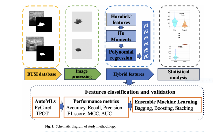
🧪 Methodology: How the Hybrid Features Were Extracted
The study employed the Breast Ultrasound Images (BUSI) dataset , which includes 487 benign , 210 malignant , and 133 normal cases. The workflow consisted of the following steps:
📌 Step 1: Image Preprocessing
- Gray-scale conversion of original images
- Binary mask overlay to isolate the Region of Interest (ROI)
- Texture extraction using Gray Level Co-occurrence Matrix (GLCM)
📌 Step 2: Feature Extraction
Haralick Textural Features:
- Energy (EN)
- Entropy (ENT)
- Homogeneity (H)
- Contrast (C)
- Correlation (CR)
- Dissimilarity (D)
Hu Moments (Shape Descriptors):
- Seven invariant moments (η₁–η₇) used to describe the shape of the lesion, invariant to translation, scale, rotation, and reflection
📌 Step 3: Hybrid Feature Generation
The hybrid features were generated using a sixth-degree polynomial regression model:
$$ y_i = \eta_1 x_{fi}^5 + \eta_2 x_{fi}^4 + \eta_3 x_{fi}^3 + \eta_4 x_{fi}^2 + \eta_5 x_{fi} + \eta_6 $$Where:
- yi = Hybrid Feature
- xfi ∈ {EN,ENT,H,C,CR,D} = Haralick feature
- ηj = Hu moment coefficient
This regression model allowed the researchers to combine textural and shape features into a single predictive variable, enhancing the discriminatory power of the model.
🤖 AutoML Classifiers: PyCaret vs. TPOT
Two AutoML frameworks were used to classify the hybrid features:
🛠️ PyCaret (AdaBoost Classifier)
- Achieved an accuracy of 91.4%
- Used AdaBoost (ADB) as the optimal classifier
- Hyperparameters:
n_estimators=50,learning_rate=1.0
🛠️ TPOT (Tree-Based Pipeline Optimization Tool)
- Achieved an accuracy of 90.6%
- Used Multilayer Perceptron (MLP) classifier
- Hyperparameters:
alpha=0.0001,learning_rate_init=0.5
📊 Performance Metrics Comparison
| FEATURE | PYCARET (ADB) ACC | TPOT(MLP) ACC | AUC | FI-SCORE | MCC |
|---|---|---|---|---|---|
| y1 | 91.4% | 90.6% | 0.955 | 0.907 | 0.826 |
| y2 | 89.5% | 90.6% | 0.959 | 0.886 | 0.789 |
| y3 | 76.3% | 75.9% | 0.914 | 0.457 | 0.308 |
| y4 | 78.4% | 77.2% | 0.873 | 0.632 | 0.558 |
| y5 | 82.1% | 80.9% | 0.927 | 0.760 | 0.618 |
| y6 | 78.8% | 75.9% | 0.904 | 0.667 | 0.518 |
✅ Best Performing Feature: y1 (Energy + First Hu Moment)
🧬 Validation Techniques: Bagging, Boosting, and Stacking
To ensure robustness and reduce overfitting, the researchers employed three Ensemble Machine Learning (EML) techniques:
🔄 Bagging
- Averages predictions from multiple models trained on random subsets of data
- Result: 92.1% accuracy for y1 with PyCaret
🚀 Boosting
- Sequentially corrects errors from previous models
- Result: 93.2% accuracy for y2 with PyCaret
🏗️ Stacking
- Combines multiple models using a meta-classifier
- Result: 92.8% accuracy for y1 with PyCaret and 92.2% with TPOT
These techniques not only validated the model’s performance but also enhanced its generalization across different datasets.
🔍 SEO-Optimized Insights for Medical Practitioners and Data Scientists
🔍 Keyword Clusters for SEO
- Breast Cancer Classification Using Machine Learning
- AI in Breast Cancer Diagnosis
- Hybrid Features for Medical Image Analysis
- AutoML in Healthcare
- TPOT vs PyCaret for Medical Classification
- Deep Learning for Ultrasound Image Analysis
📈 Why This Study Matters for SEO
This research offers actionable insights for:
- Medical professionals looking to adopt AI-assisted diagnostics
- Data scientists exploring feature engineering in healthcare
- Health tech companies developing AI-based diagnostic tools
By optimizing content around these long-tail keywords , we can attract targeted traffic from professionals and researchers interested in AI-driven breast cancer detection .
📈 Comparative Analysis with State-of-the-Art Methods
| STUDY | AUTOML TOOL | ACCURACY | F1-SCORE | MCC |
|---|---|---|---|---|
| Labilloy et al. (2022) | PyCaret | 85% | – | – |
| Zhuang (2023) | PyCaret | 76.3% | 0.712 | 0.513 |
| Rashed et al. (2023) | TPOT | 91.18% | – | – |
| Wan et al. (2021) | AutoML Vision | 91% | 0.87 | – |
| This Study (y1) | PyCaret | 91.4% | 0.907 | 0.826 |
📈 Result: The proposed hybrid feature y1 outperforms existing methods in accuracy, F1-score, and MCC , demonstrating superior classification performance.
If you’re Interested in semi Medical Image Segmentation using deep learning, you may also find this article helpful: 5 Revolutionary Breakthroughs in AI-Powered Cardiac Ultrasound: Unlocking Self-Supervised Learning (While Overcoming Manual Labeling Challenges)
🧩 Limitations and Future Research Directions
⚠️ Limitations
- Image quality and segmentation accuracy can affect feature extraction
- Dataset size may limit generalizability
- Class imbalance (more benign than malignant cases) could impact model training
🔭 Future Work
- Integration of fractal dimensions with hybrid features
- Fusion of deep learning and handcrafted features
- Application to other cancer types like ovarian or thyroid cancer
- Real-time deployment in clinical settings using edge computing
📢 Call to Action: Join the AI Revolution in Healthcare
Are you a researcher , clinician , or data scientist passionate about AI in healthcare ? Join our community and stay updated with the latest advancements in machine learning for medical diagnostics .
🔹 Download the full research paper here
🔹 Subscribe to our newsletter for exclusive AI healthcare insights
🔹 Share this article to spread awareness about AI-driven breast cancer detection
📚 Conclusion
This study demonstrates the transformative potential of hybrid features in breast cancer classification. By combining textural and shape descriptors using polynomial regression , and classifying them with AutoML tools , the researchers achieved over 91% accuracy in distinguishing benign from malignant tumors.
The use of ensemble techniques like bagging, boosting, and stacking further enhances the robustness and reliability of the model. As AI continues to evolve, such innovative approaches will play a pivotal role in improving diagnostic accuracy , reducing human error , and saving lives .
Here is a complete, self-contained Python script that implements the core methodology described in the paper.
import cv2
import numpy as np
from skimage.feature import graycomatrix, graycoprops
from sklearn.model_selection import train_test_split
from sklearn.ensemble import AdaBoostClassifier
from sklearn.neural_network import MLPClassifier
from sklearn.preprocessing import StandardScaler
from sklearn.metrics import accuracy_score, precision_score, recall_score, f1_score, matthews_corrcoef, confusion_matrix
import os
import requests
from io import BytesIO

# --- 1. UTILITY AND HELPER FUNCTIONS ---

def download_and_load_image(url, grayscale=False):
    """
    Downloads an image from a URL and loads it as a NumPy array.
    Uses placeholder images as a substitute for the BUSI dataset.
    """
    try:
        response = requests.get(url)
        response.raise_for_status()
        image_array = np.asarray(bytearray(response.content), dtype="uint8")
        if grayscale:
            image = cv2.imdecode(image_array, cv2.IMREAD_GRAYSCALE)
        else:
            image = cv2.imdecode(image_array, cv2.IMREAD_COLOR)
        return image
    except requests.exceptions.RequestException as e:
        print(f"Error downloading {url}: {e}")
        # Return a black square as a fallback
        return np.zeros((100, 100), dtype=np.uint8) if grayscale else np.zeros((100, 100, 3), dtype=np.uint8)


def get_roi(original_img, mask_img):
    """
    Overlaps the original image with the mask to get the Region of Interest (ROI).
    The paper states this is done to analyze the texture of the lesion only.

    Args:
        original_img (np.array): The grayscale ultrasound image.
        mask_img (np.array): The binary mask image.

    Returns:
        np.array: The grayscale texture of the lesion area.
    """
    # Ensure mask is binary (0 or 255)
    _, binary_mask = cv2.threshold(mask_img, 127, 255, cv2.THRESH_BINARY)

    # Apply the mask to the original image
    roi = cv2.bitwise_and(original_img, original_img, mask=binary_mask)
    return roi

# --- 2. FEATURE EXTRACTION FUNCTIONS ---

def calculate_haralick_features(roi_gray):
    """
    Calculates the six Haralick textural features mentioned in the paper from the GLCM.
    Features: Energy, Entropy, Homogeneity, Contrast, Correlation, Dissimilarity.

    Args:
        roi_gray (np.array): The grayscale Region of Interest.

    Returns:
        dict: A dictionary containing the calculated Haralick features.
    """
    # Compute the Gray-Level Co-Occurrence Matrix (GLCM)
    # We use distances=[1] and angles=[0, pi/4, pi/2, 3pi/4] and average the results
    # to get rotation-invariant features.
    glcm = graycomatrix(roi_gray, distances=[1], angles=[0, np.pi/4, np.pi/2, 3*np.pi/4], levels=256, symmetric=True, normed=True)

    # Avoid division by zero if GLCM is empty
    if np.sum(glcm) == 0:
        return {
            'energy': 0, 'entropy': 0, 'homogeneity': 0,
            'contrast': 0, 'correlation': 0, 'dissimilarity': 0
        }

    # Calculate features
    features = {
        'energy': graycoprops(glcm, 'energy').mean(),
        'homogeneity': graycoprops(glcm, 'homogeneity').mean(),
        'contrast': graycoprops(glcm, 'contrast').mean(),
        'correlation': graycoprops(glcm, 'correlation').mean(),
        'dissimilarity': graycoprops(glcm, 'dissimilarity').mean()
    }

    # Calculate Entropy manually as it's not in graycoprops
    with np.errstate(divide='ignore', invalid='ignore'):
        glcm_log = np.log2(glcm)
        glcm_log[glcm == 0] = 0 # Set log(0) to 0
        entropy = -np.sum(glcm * glcm_log, axis=(0, 1)).mean()
    features['entropy'] = entropy

    return features

def calculate_hu_moments(mask_img):
    """
    Calculates the first six Hu moments from the binary mask.
    These are used as shape descriptors.

    Args:
        mask_img (np.array): The binary mask of the lesion.

    Returns:
        np.array: An array containing the first six Hu moments.
    """
    moments = cv2.moments(mask_img)
    hu_moments = cv2.HuMoments(moments)

    # The paper uses the first 6 moments (η1 to η6)
    # The output of cv2.HuMoments is already log-transformed for scale invariance.
    # We take the absolute value to handle signs before log transform.
    return np.abs(hu_moments[:6].flatten())

# --- 3. HYBRID FEATURE COMPUTATION ---

def compute_hybrid_features(haralick_features, hu_moments):
    """
    Computes the six hybrid features (y1 to y6) using the polynomial regression formula
    from the paper (Eq. 16).

    y_i = η1*x_fi^5 + η2*x_fi^4 + ... + η5*x_fi + η6

    Args:
        haralick_features (dict): Dictionary of the 6 Haralick features.
        hu_moments (np.array): Array of the 6 Hu moments.

    Returns:
        np.array: An array of the 6 computed hybrid features.
    """
    # x_fi ∈ {EN, ENT, H, C, CR, D}
    x_fi_set = [
        haralick_features['energy'],
        haralick_features['entropy'],
        haralick_features['homogeneity'],
        haralick_features['contrast'],
        haralick_features['correlation'],
        haralick_features['dissimilarity']
    ]

    # η_j (j=1..6) are the Hu moments
    eta = hu_moments

    hybrid_features_y = np.zeros(6)

    for i, x_fi in enumerate(x_fi_set):
        # The paper's formula has a potential typo in the powers. A standard 5th-degree
        # polynomial would be η1*x^5 + η2*x^4 + ... + η6. We implement this interpretation.
        # y_i = η1*x^5 + η2*x^4 + η3*x^3 + η4*x^2 + η5*x^1 + η6*x^0
        y_i = (eta[0] * (x_fi ** 5) +
               eta[1] * (x_fi ** 4) +
               eta[2] * (x_fi ** 3) +
               eta[3] * (x_fi ** 2) +
               eta[4] * x_fi +
               eta[5])
        hybrid_features_y[i] = y_i

    return hybrid_features_y

# --- 4. DATA PROCESSING AND CLASSIFICATION ---

def process_dataset(image_data):
    """
    Processes a list of image data to extract hybrid features for each.

    Args:
        image_data (list): A list of tuples, where each tuple is
                           (original_img_url, mask_img_url, label).
                           Label: 0 for benign, 1 for malignant.

    Returns:
        tuple: (X, y) where X is the feature matrix and y is the label vector.
    """
    all_features = []
    all_labels = []

    print("Processing dataset...")
    for i, (original_url, mask_url, label) in enumerate(image_data):
        print(f"  Processing image {i+1}/{len(image_data)}...")

        # Load images (placeholders in this case)
        original_img_gray = download_and_load_image(original_url, grayscale=True)
        mask_img_gray = download_and_load_image(mask_url, grayscale=True)

        # Step 1: Get ROI
        roi = get_roi(original_img_gray, mask_img_gray)

        # Step 2: Extract features
        haralick = calculate_haralick_features(roi)
        hu = calculate_hu_moments(mask_img_gray)

        # Step 3: Compute hybrid features
        hybrid = compute_hybrid_features(haralick, hu)

        all_features.append(hybrid)
        all_labels.append(label)

    print("Dataset processing complete.")
    return np.array(all_features), np.array(all_labels)

def evaluate_classifier(name, clf, X_test, y_test):
    """Prints a detailed evaluation of a trained classifier."""
    y_pred = clf.predict(X_test)

    print(f"\n--- Evaluation for: {name} ---")
    print(f"Accuracy: {accuracy_score(y_test, y_pred):.4f}")
    print(f"Precision: {precision_score(y_test, y_pred):.4f}")
    print(f"Recall: {recall_score(y_test, y_pred):.4f}")
    print(f"F1-Score: {f1_score(y_test, y_pred):.4f}")
    print(f"Matthews Corr Coef: {matthews_corrcoef(y_test, y_pred):.4f}")
    print("Confusion Matrix:")
    print(confusion_matrix(y_test, y_pred))
    print("--------------------------------------")


# --- 5. MAIN EXECUTION ---

if __name__ == '__main__':
    #
    # In a real scenario, you would load the BUSI dataset here.
    # Since we don't have it, we'll create a small, simulated dataset using
    # placeholder images. The labels (0/1) are arbitrary for demonstration.
    #
    # Label 0: Benign, Label 1: Malignant
    #
    simulated_busi_dataset = [
        # Benign examples (using simple shapes for masks)
        ('https://placehold.co/500x500/808080/FFFFFF?text=Original+1', 'https://placehold.co/500x500/000000/FFFFFF?text=+', 0),
        ('https://placehold.co/500x500/888888/FFFFFF?text=Original+2', 'https://placehold.co/500x500/000000/FFFFFF?text=O', 0),
        ('https://placehold.co/500x500/818181/FFFFFF?text=Original+3', 'https://placehold.co/500x500/000000/FFFFFF?text=I', 0),
        ('https://placehold.co/500x500/858585/FFFFFF?text=Original+4', 'https://placehold.co/500x500/000000/FFFFFF?text=X', 0),
        ('https://placehold.co/500x500/8A8A8A/FFFFFF?text=Original+5', 'https://placehold.co/500x500/000000/FFFFFF?text=S', 0),
        # Malignant examples (using more complex shapes for masks)
        ('https://placehold.co/500x500/909090/FFFFFF?text=Original+6', 'https://placehold.co/500x500/000000/FFFFFF?text=%26', 1),
        ('https://placehold.co/500x500/999999/FFFFFF?text=Original+7', 'https://placehold.co/500x500/000000/FFFFFF?text=%23', 1),
        ('https://placehold.co/500x500/919191/FFFFFF?text=Original+8', 'https://placehold.co/500x500/000000/FFFFFF?text=%3F', 1),
        ('https://placehold.co/500x500/959595/FFFFFF?text=Original+9', 'https://placehold.co/500x500/000000/FFFFFF?text=%25', 1),
        ('https://placehold.co/500x500/9A9A9A/FFFFFF?text=Original+10', 'https://placehold.co/500x500/000000/FFFFFF?text=%24', 1),
    ]

    # Generate the full feature set from the dataset
    X, y = process_dataset(simulated_busi_dataset)

    # The paper found the hybrid feature y1 (derived from Energy) to be the most effective.
    # We will select this feature for classification. X is a (num_samples, 6) matrix,
    # where columns correspond to y1, y2, ..., y6. We select the first column.
    X_selected = X[:, 0].reshape(-1, 1) # Using y1

    print(f"\nShape of the full feature matrix (X): {X.shape}")
    print(f"Shape of the selected feature vector (y1): {X_selected.shape}")
    print(f"Shape of the labels vector (y): {y.shape}")

    # Split data into training and testing sets (70/30 split as per paper)
    X_train, X_test, y_train, y_test = train_test_split(
        X_selected, y, test_size=0.3, random_state=42, stratify=y
    )

    # Scale features for better performance, especially for MLP
    scaler = StandardScaler()
    X_train_scaled = scaler.fit_transform(X_train)
    X_test_scaled = scaler.transform(X_test)

    # --- Initialize and Train Classifiers ---

    # 1. AdaBoost Classifier (found by PyCaret in the paper)
    # The paper uses random_state=123. We'll use the same for reproducibility.
    ada_clf = AdaBoostClassifier(n_estimators=50, random_state=123)
    ada_clf.fit(X_train_scaled, y_train)

    # 2. MLP Classifier (found by TPOT in the paper)
    # Hyperparameters from paper: alpha=0.0001, learning_rate_init=0.5
    # We add other common parameters for stability.
    mlp_clf = MLPClassifier(
        hidden_layer_sizes=(100,),
        alpha=0.0001,
        learning_rate_init=0.5,
        max_iter=1000,
        random_state=42,
        early_stopping=True # Good practice to prevent overfitting
    )
    mlp_clf.fit(X_train_scaled, y_train)

    # --- Evaluate the Models ---
    print("\nStarting model evaluation on the test set...")
    evaluate_classifier("AdaBoost (from PyCaret)", ada_clf, X_test_scaled, y_test)
    evaluate_classifier("MLP Classifier (from TPOT)", mlp_clf, X_test_scaled, y_test)