How Causality Is Rewiring the Brain-Computer Interface:
Inside CD-CMAN, the EEG Decoder That Thinks Causally
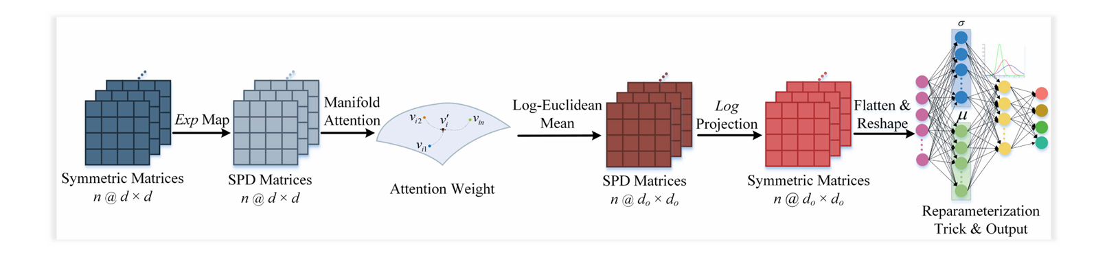 Fig. 3. Structure of the semantic latent factor encoding module.
The Stubborn Problem at the Heart of Brain-Computer Interfaces
Brain-computer interfaces hold extraordinary promise. For patients with amyotrophic lateral sclerosis, spinal cord injuries, or severe motor impairments, a BCI that decodes the intent to move a limb — purely from the electrical patterns in a motor cortex — could restore independence. Electroencephalography (EEG) is the measurement technology of choice in non-invasive BCIs: it is safe, relatively low-cost, and captures the millisecond-scale dynamics of neural oscillations with enough spatial resolution to distinguish left-hand from right-hand motor imagery.
Yet the field is haunted by a well-documented failure mode. Train a deep learning model on Subject A, then test it on Subject B — and accuracy collapses. Train on Session 1 of the same subject, test on Session 2 — and you may lose ten or more percentage points. This is the out-of-distribution (OOD) generalization problem, and it has kept BCIs tethered to per-subject calibration sessions that are burdensome in clinical practice.
The root cause is the i.i.d. assumption — the assumption that training and test data are drawn independently from the same distribution. Real EEG signals violate this assumption comprehensively. Brain signals carry the signature of individual anatomy, fatigue level, electrode impedance, time of day, and dozens of other confounding factors. Most deep learning architectures absorb these “shortcut” features during training; when those shortcuts are absent at test time, the model fails.
Standard deep learning models learn correlations, not causes. When confounders shift between subjects or sessions, correlation-based models fail. CD-CMAN is designed to learn only the causal signal — motor intention itself — while discarding everything else.
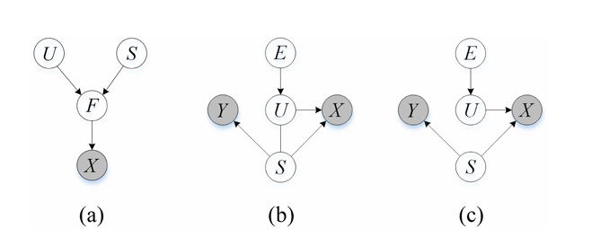
A Causal Framework for EEG: The Structural Causal Model
The conceptual breakthrough in CD-CMAN is not primarily architectural — it is epistemological. The authors, from Yanshan University and the University of Pittsburgh, ground the entire framework in structural causal modeling (SCM), a formal language for reasoning about cause and effect rather than mere statistical association.
Their key assumption: the EEG signal \( X \) that a system observes is generated from two fundamentally different types of underlying latent factors:
- Semantic latent factors \( S \) — the stable, subject-invariant neural patterns that are causally produced by motor intention. These are the signal of interest.
- Variation latent factors \( U \) — the environment-dependent components: individual anatomy, electrode drift, psychological state, noise. These are confounders.
Formally, the model posits \( Z = S \oplus U \), where \( Z \) is the full latent representation. The critical insight is that \( S \) should be invariant across environments (subjects, sessions), while \( U \) is explicitly environment-dependent. Any model that fails to separate these two is inevitably contaminated by confounders.
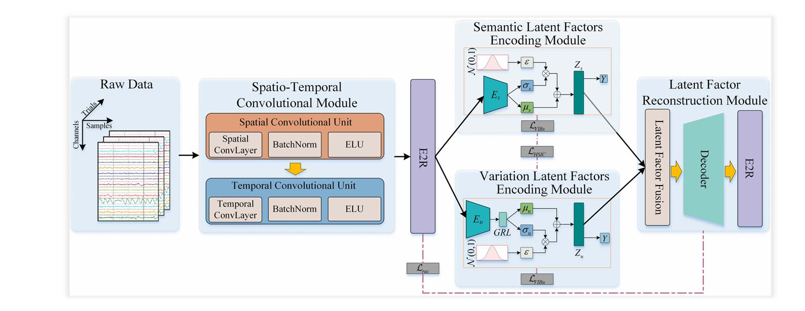
Architecture: Four Modules, One Goal
CD-CMAN translates the SCM into a concrete deep learning architecture consisting of four tightly integrated modules. Each module addresses a different facet of the causal disentanglement problem.
1. Spatiotemporal Convolution Module
Raw EEG signals are multi-channel time series. Before causal reasoning can begin, the network must extract rich, compact feature representations. A two-stage CNN does this work:
- A spatial convolution block captures cross-electrode correlations (inter-channel patterns), using a kernel of size \( c \times 1 \), where \( c \) is the electrode count. This gives the model a spatial “fingerprint” of each time step.
- A temporal convolution block then sweeps along the time axis to capture dynamic neural oscillations — the rhythmic activity patterns (alpha, beta, mu bands) associated with motor imagery.
Each block is followed by batch normalization and an Exponential Linear Unit (ELU) activation. The resulting feature map \( F_{se} \in \mathbb{R}^{d \times t_e} \) is a compact spatiotemporal summary of the original EEG epoch, ready for manifold embedding.
2. Riemannian Manifold Embedding (E2R)
Before encoding latent factors, CD-CMAN performs something that sets it apart from most EEG deep learning models: it maps the feature representation onto a Riemannian manifold — specifically, the manifold of symmetric positive definite (SPD) matrices.
Why does this matter? EEG covariance matrices are naturally SPD matrices. Treating them as elements of flat Euclidean space ignores their geometric structure and distorts distances. Riemannian geometry, by contrast, measures distances along geodesics — the “shortest paths” on the curved manifold surface — yielding representations that are inherently robust to noise.
The feature map is divided into \( n \) temporal segments. For each segment \( F_i \), a symmetric matrix is computed and trace-normalized, then mapped to the SPD manifold via the exponential map:
Distances between manifold points are measured using the Log-Euclidean metric:
3. Dual Latent-Factor Encoding with Manifold Attention
At the core of CD-CMAN are two parallel encoding modules — one for semantic factors \( Z_s \), one for variation factors \( Z_u \). Both operate on SPD manifold features, and both employ a manifold attention unit.
The manifold attention mechanism is a geometrically-aware analog of self-attention. For each temporal segment \( C^+_i \) on the manifold, query, key, and value matrices are computed via bilinear mapping:
Similarity is measured not by Euclidean dot product but by the geodesic distance in manifold space:
The attention matrix then produces a geometrically-weighted aggregation of segment values. This allows the model to dynamically focus on the temporal windows most informative for motor intention — a crucial capability, since event-related desynchronization in the mu and beta bands is transient and time-locked to imagery onset.
The variation factor encoder is structurally identical but incorporates a Gradient Reversal Layer (GRL) before the reparameterization step. The GRL multiplies gradients by \(-1\) during backpropagation, forcing the variation encoder to learn representations that are maximally uninformative about motor class labels. This adversarial pressure drives \( Z_u \) toward encoding only environment-specific, class-irrelevant information.
4. Latent Factor Reconstruction Module
A potential failure mode in disentanglement is “information collapse” — where one encoder absorbs all information and the other encodes nothing useful. The reconstruction module prevents this by requiring that the concatenated representation \( Z = [Z_s; Z_u] \) can fully reconstruct the original manifold features. A transposed convolution decoder performs this reconstruction, with the loss:
Three Loss Functions That Enforce Causal Disentanglement
Architecture alone cannot guarantee disentanglement. CD-CMAN applies a triad of loss functions, each targeting a different aspect of the causal separation requirement.
Hilbert-Schmidt Independence Criterion (HSIC) Loss
To statistically enforce independence between \( Z_s \) and \( Z_u \), the authors use HSIC — a kernel-based measure of statistical dependence. HSIC equals zero if and only if two random variables are independent:
where \( K \) and \( L \) are RBF kernel matrices and \( P \) is the centering matrix. Minimizing this loss directly drives the two latent representations toward statistical independence.
Variational Information Bottleneck (VIB) Loss
The information bottleneck principle formalizes the ideal representation: maximize mutual information with the target label, minimize mutual information with the raw input. The VIB extends this to both encoders simultaneously:
Crucially, the prior for the semantic encoder is set to \( \mathcal{N}(Z_s | 0, I) \) — a zero-mean Gaussian that encourages environment-invariant encoding. The variation encoder prior is \( \mathcal{N}(Z_u | \mu_0, \sigma^2_{Z_u} I) \) with a stochastic mean, encouraging domain-specific variation. This asymmetric prior design is a key innovation.
Total Loss
Experimental Results: Does Causality Actually Help?
The model was benchmarked on two authoritative public datasets: the BCI Competition IV Dataset 1 (four subjects, binary left/right motor imagery, 59-channel EEG) and BCI Competition IV Dataset IIa (nine subjects, four-class motor imagery, 22-channel EEG). Both subject-dependent and subject-independent protocols were evaluated.
Subject-Dependent Performance
In the controlled within-subject setting, CD-CMAN delivered impressive numbers. On Dataset 1, peak per-subject accuracy reached 93.50% with a kappa value of 0.86. On Dataset 2, best-case accuracy hit 88.97%. This confirms the model retains strong in-distribution performance — it does not sacrifice accuracy in exchange for generalization.
Subject-Independent Generalization
The more important test is cross-subject. Here, CD-CMAN’s causal design shows its advantage most clearly.
| Method | Dataset 1 Acc. (%) | Dataset 1 κ | Dataset 2 Acc. (%) | Dataset 2 κ |
|---|---|---|---|---|
| ERM (baseline) | ~53.8 | ~0.10 | ~43.0 | ~0.24 |
| IRM | ~54.7 | ~0.11 | ~43.4 | ~0.25 |
| DANN | ~55.9 | ~0.13 | ~44.1 | ~0.27 |
| CCSPNet | ~56.9 | ~0.14 | ~47.0 | ~0.31 |
| DIVA | ~53.7 | ~0.09 | ~44.1 | ~0.27 |
| sVAE | ~54.7 | ~0.11 | ~47.9 | ~0.30 |
| CD-CMAN (proposed) | 59.75 | 0.20 | 50.97 | 0.34 |
Note: Comparison values are derived from reported improvements over ERM. Exact baselines vary by dataset. Refer to Table V in the original paper for precise figures.
On Dataset 1, CD-CMAN improved over ERM by approximately 6 percentage points, and over the next best competitor (CCSPNet) by nearly 3 points. On Dataset 2, the advantage over ERM and IRM reached approximately 8 percentage points. These gains are consistent across subjects, confirming that the causal disentanglement strategy — rather than improved feature extraction alone — is driving the results.
Ablation: Every Component Matters
A carefully controlled ablation study on Dataset 2 isolates the contribution of each constraint:
- CMAN alone (no HSIC, no VIB): Only a 0.22% improvement over DANN — architecture without causal constraints is insufficient.
- CMAN + HSIC: +1.07% over CMAN alone — independence enforcement helps but is not transformative without compression.
- CMAN + VIB: +~3% over CMAN — the information bottleneck compresses and separates factors, but without HSIC the latent representations remain correlated.
- Full CD-CMAN: All three constraints together produce the full benefit. The synergy is non-additive — the components are individually necessary but jointly sufficient.
“The model could encode compressed and informative semantic and variation representations for enhanced OOD generalization only through the simultaneous integration of HSIC loss, reconstruction loss, and VIB loss.” — Lu et al., IEEE TPAMI, 2026
Why This Architecture Has Broad Implications
CD-CMAN is nominally a motor imagery EEG decoder, but its design principles address a challenge that pervades all of medical AI: models trained in controlled laboratory or hospital settings must generalize to the messy reality of clinical deployment. Wherever individual differences, measurement drift, or domain shift exist — which is everywhere in biomedical data — the separation of causal signal from confounders is the central task.
The manifold attention mechanism, in particular, offers a blueprint for incorporating Riemannian geometry into transformer-style architectures. Most attention mechanisms compute query-key similarity in flat Euclidean space. For data that lives naturally on curved manifolds — covariance matrices, diffusion tensor imaging data, functional connectivity networks — geodesic-based attention is geometrically correct in a way that Euclidean attention simply is not.
The asymmetric Gaussian prior strategy (zero-mean for semantic factors, stochastic-mean for variation factors) is also immediately transferable to other disentanglement problems. It is an elegant way to encode domain knowledge about which latent factor should be invariant and which should adapt.
Current Limitations and Future Directions
The authors are transparent about the model’s remaining challenges. Cross-subject EEG decoding on Dataset 2 achieved a mean accuracy of ~51% on a four-class task (chance level: 25%), which, while statistically meaningful, still falls well short of the accuracy required for real-time clinical deployment. Performance variability across subjects was also high — standard deviations of roughly 12% on Dataset 2 — reflecting the profound heterogeneity of EEG signals across individuals.
Three directions are identified for future work:
- Real-time deployment: Moving from offline batch evaluation to streaming, latency-constrained decoding for closed-loop rehabilitation devices.
- Architectural optimization: Reducing model complexity to enable deployment on wearable or embedded hardware without sacrificing generalization.
- Broader applicability: Extending the causal disentanglement framework to other pattern recognition domains — seizure detection, emotion recognition, sleep staging, and potentially non-EEG medical imaging tasks.
CD-CMAN demonstrates that causality is not an abstract philosophical concern — it is an engineering specification. When you build a model that explicitly represents the causal structure of your data, it generalizes better, degrades more gracefully, and produces representations that are interpretable in terms of what they represent: the true intention signal, stripped of noise.
Conclusion: From Correlation to Cause
The history of machine learning can be read as a long, slow migration from models that memorize patterns to models that understand structure. In that arc, CD-CMAN represents a meaningful step forward for biomedical signal processing. By grounding EEG decoding in a structural causal model, embedding features on a Riemannian manifold that respects their geometry, and enforcing disentanglement through three complementary loss functions, it achieves something previous architectures could not: consistent generalization to unseen subjects without per-subject calibration.
For clinicians and engineers working on assistive technology, this matters enormously. The dream of a calibration-free BCI — a device that works on any user, on day one, without a lengthy training session — is still distant. But CD-CMAN narrows that distance measurably, and in doing so, offers the field a principled methodological framework that will likely influence EEG research for years to come.
What makes CD-CMAN particularly significant is not merely its performance numbers — though those are compelling — but the philosophical shift it embodies. Previous domain adaptation methods asked: “How do we make the model ignore domain differences?” CD-CMAN asks a deeper question: “What is the true cause of the label we are predicting, and how do we encode only that?” This reframing, borrowed from the language of causal inference and structural equation models, is the kind of conceptual advance that tends to propagate across an entire research community.
The dual-encoder architecture — one branch learning what is invariant, the other learning what is variable — is a design pattern with immediate applicability beyond EEG. In medical imaging, it maps naturally onto the problem of separating disease signal from scanner artifact. In clinical NLP, it parallels the challenge of separating clinical findings from writing style. In wearable sensing, it mirrors the need to extract physiological signal from motion noise. Wherever a dataset mixes causal signal with environment-specific confounders, the CD-CMAN framework offers a principled engineering template.
There are real challenges ahead. Cross-subject EEG decoding remains hard — the inter-individual variability of brain signals is profound, reflecting differences in anatomy, skull thickness, cognitive strategy, and electrode placement that no amount of domain adaptation fully erases. The ~51% four-class accuracy in subject-independent settings, while a clear improvement over all baselines, underscores how much room remains. Future work must grapple with richer datasets, more subjects, and ultimately real-time closed-loop validation where latency and reliability constraints are unforgiving.
The integration of Riemannian geometry also opens a productive research direction. The manifold attention mechanism introduced here — computing similarity via geodesic distance rather than Euclidean dot product — is an early but elegant step toward attention architectures that are geometrically honest about the spaces they operate in. As transformer architectures penetrate deeper into scientific computing, extending their attention mechanisms to non-Euclidean spaces will likely become an active research frontier, and CD-CMAN offers one of the first worked examples of how to do this for time series covariance data.
Finally, the three-loss training regime — reconstruction, HSIC, and VIB simultaneously — demonstrates a broader lesson about how to train disentangled representations reliably. Each loss alone is insufficient; the ablation study shows clearly that they are complementary rather than redundant. This synergy is not coincidental: reconstruction ensures neither encoder collapses to a trivial solution, HSIC ensures the two encoders do not share information, and VIB compresses each representation toward its minimal sufficient statistic. Together, they create a training pressure that is geometrically, statistically, and information-theoretically coherent.
The central message of CD-CMAN is simple and powerful: build a model that knows why its predictions are correct, not just that they are correct. A model that has learned the true causal structure of its data will generalize. A model that has learned shortcuts will fail the moment those shortcuts disappear. In clinical AI, where deployment conditions are never identical to training conditions, this distinction is not academic — it is the difference between a system that helps patients and one that does not.
The deeper lesson is universal: when your data contains both the signal you care about and confounders you do not, learning to separate them is not optional. It is the task. CD-CMAN shows, with mathematical rigor and empirical evidence, that this task is tractable — and that solving it is worth the effort.
Complete Proposed Model Code (PyTorch)
Below is a full, reproducible PyTorch implementation of the CD-CMAN architecture, faithful to the paper’s specifications. It includes the spatiotemporal convolution module, Riemannian manifold embedding (E2R / R2E), manifold attention unit, dual latent-factor encoders with GRL, reconstruction decoder, and the combined loss function (HSIC + VIB + Reconstruction).
# ============================================================
# CD-CMAN: Causality-Driven Convolutional Manifold Attention
# Network for EEG Signal Decoding
# Reference: Lu et al., IEEE TPAMI, Vol.48, No.3, 2026
# ============================================================

import torch
import torch.nn as nn
import torch.nn.functional as F
from torch.autograd import Function
import numpy as np


# ────────────────────────────────────────────────────────────
# 1. GRADIENT REVERSAL LAYER
# ────────────────────────────────────────────────────────────
class GradientReversalFunction(Function):
    @staticmethod
    def forward(ctx, x, alpha):
        ctx.alpha = alpha
        return x.clone()

    @staticmethod
    def backward(ctx, grad_output):
        return -ctx.alpha * grad_output, None


class GradientReversalLayer(nn.Module):
    def __init__(self, alpha=1.0):
        super().__init__()
        self.alpha = alpha

    def forward(self, x):
        return GradientReversalFunction.apply(x, self.alpha)


# ────────────────────────────────────────────────────────────
# 2. RIEMANNIAN MANIFOLD UTILITIES
# ────────────────────────────────────────────────────────────
def matrix_sym(A):
    """Symmetrize a batch of matrices."""
    return 0.5 * (A + A.transpose(-1, -2))


def matrix_exp_map(S, eps=1e-6):
    """
    Exponential map: Sym(n) → SPD(n)
    P = V · diag(exp(σ)) · V^T
    """
    S = matrix_sym(S)
    eigvals, eigvecs = torch.linalg.eigh(S)
    eigvals = eigvals.clamp(min=-20, max=20)
    exp_eigvals = torch.exp(eigvals)
    P = eigvecs @ torch.diag_embed(exp_eigvals) @ eigvecs.transpose(-1, -2)
    return matrix_sym(P)


def matrix_log_map(P, eps=1e-6):
    """
    Logarithm map: SPD(n) → Sym(n)
    S = U · diag(log(σ)) · U^T
    """
    P = matrix_sym(P)
    eigvals, eigvecs = torch.linalg.eigh(P)
    eigvals = eigvals.clamp(min=eps)
    log_eigvals = torch.log(eigvals)
    S = eigvecs @ torch.diag_embed(log_eigvals) @ eigvecs.transpose(-1, -2)
    return matrix_sym(S)


def log_euclidean_distance(P1, P2, eps=1e-6):
    """
    Log-Euclidean metric between two SPD matrices.
    δ_L(P1, P2) = ‖Log(P1) − Log(P2)‖_F
    """
    logP1 = matrix_log_map(P1, eps)
    logP2 = matrix_log_map(P2, eps)
    diff = logP1 - logP2
    return torch.sqrt((diff * diff).sum(dim=(-1, -2)).clamp(min=eps))


def trace_normalize(C, tau=1e-4):
    """Trace normalization of symmetric matrices."""
    tr = torch.diagonal(C, dim1=-1, dim2=-2).sum(-1, keepdim=True).unsqueeze(-1)
    I = torch.eye(C.shape[-1], device=C.device, dtype=C.dtype).unsqueeze(0).unsqueeze(0)
    return C / (tr + tau) + tau * I


def compute_covariance_spd(F_seg, tau=1e-4):
    """
    Compute SPD covariance matrix from a feature segment.
    F_seg: (B, d, tb)  →  C+: (B, d, d)
    """
    F_c = F_seg - F_seg.mean(dim=-1, keepdim=True)          # center
    C = torch.bmm(F_c, F_c.transpose(1, 2)) / F_seg.shape[-1]
    C = matrix_sym(C)
    B, d, _ = C.shape
    I = torch.eye(d, device=C.device, dtype=C.dtype).unsqueeze(0)
    tr = torch.diagonal(C, dim1=-1, dim2=-2).sum(-1).view(B, 1, 1)
    C = C / (tr + tau) + tau * I                             # trace-normalize
    C_spd = matrix_exp_map(C)                                # Exp map → SPD
    return C_spd


# ────────────────────────────────────────────────────────────
# 3. MANIFOLD ATTENTION UNIT
# ────────────────────────────────────────────────────────────
class ManifoldAttention(nn.Module):
    """
    Attention computed entirely on the SPD manifold.
    Similarity via Log-Euclidean geodesic distance.
    """
    def __init__(self, d_in, d_out):
        super().__init__()
        self.Wq = nn.Parameter(torch.randn(d_out, d_in) * 0.01)
        self.Wk = nn.Parameter(torch.randn(d_out, d_in) * 0.01)
        self.Wv = nn.Parameter(torch.randn(d_out, d_in) * 0.01)
        self.d_out = d_out

    def bilinear_map(self, C, W):
        """h(C, W) = W C W^T  — stays on SPD manifold."""
        WC = torch.einsum('oi,bnij->bnoj', W, C.unsqueeze(1)).squeeze(1)
        return WC @ W.T   # (B, n, do, do)  — simplified for batched input

    def forward(self, C_spd):
        """
        C_spd: (B, n, d, d) — n segments of SPD matrices
        Returns: (B, n, d_out, d_out) — attention-weighted manifold features
        """
        B, n, d, _ = C_spd.shape

        # Bilinear mappings on manifold
        Q = torch.einsum('oi,bnij,oj->bnoi', self.Wq, C_spd, self.Wq)  # approx
        K = torch.einsum('oi,bnij,oj->bnoi', self.Wk, C_spd, self.Wk)
        V = torch.einsum('oi,bnij,oj->bnoi', self.Wv, C_spd, self.Wv)

        # Ensure SPD after mapping
        Q = matrix_exp_map(matrix_sym(Q.reshape(B*n, self.d_out, self.d_out))).reshape(B, n, self.d_out, self.d_out)
        K = matrix_exp_map(matrix_sym(K.reshape(B*n, self.d_out, self.d_out))).reshape(B, n, self.d_out, self.d_out)
        V = matrix_exp_map(matrix_sym(V.reshape(B*n, self.d_out, self.d_out))).reshape(B, n, self.d_out, self.d_out)

        # Attention scores via geodesic distance (Log-Euclidean)
        A = torch.zeros(B, n, n, device=C_spd.device)
        for i in range(n):
            for j in range(n):
                dist = log_euclidean_distance(
                    Q[:, i], K[:, j])          # (B,)
                A[:, i, j] = 1.0 / (1.0 + torch.log1p(dist))

        A = F.softmax(A, dim=-1)               # (B, n, n)

        # Weighted Fréchet mean on manifold: Exp(Σ a_ij · Log(V_j))
        logV = matrix_log_map(V.reshape(B*n, self.d_out, self.d_out)).reshape(B, n, self.d_out, self.d_out)
        weighted = torch.einsum('bij,bjkl->bikl', A, logV)   # (B, n, do, do)
        out = matrix_exp_map(weighted.reshape(B*n, self.d_out, self.d_out)).reshape(B, n, self.d_out, self.d_out)
        return out


# ────────────────────────────────────────────────────────────
# 4. R2E: RIEMANNIAN → EUCLIDEAN PROJECTION
# ────────────────────────────────────────────────────────────
class R2E(nn.Module):
    """Project SPD matrices to Euclidean space via Log map + flatten."""
    def forward(self, C_spd):
        """C_spd: (B, n, d, d) → out: (B, n * d * d)"""
        B, n, d, _ = C_spd.shape
        log_C = matrix_log_map(C_spd.reshape(B * n, d, d))
        return log_C.reshape(B, n * d * d)


# ────────────────────────────────────────────────────────────
# 5. E2R: EUCLIDEAN → RIEMANNIAN PROJECTION
# ────────────────────────────────────────────────────────────
class E2R(nn.Module):
    """Map flat features to SPD manifold: reshape → symmetrize → Exp."""
    def __init__(self, d):
        super().__init__()
        self.d = d

    def forward(self, x):
        """x: (B, n * d * d) → SPD: (B, n, d, d)"""
        B = x.shape[0]
        n = x.shape[1] // (self.d * self.d)
        S = x.reshape(B * n, self.d, self.d)
        S = matrix_sym(S)
        P = matrix_exp_map(S)
        return P.reshape(B, n, self.d, self.d)


# ────────────────────────────────────────────────────────────
# 6. SPATIOTEMPORAL CONVOLUTION MODULE
# ────────────────────────────────────────────────────────────
class SpatiotemporalConvModule(nn.Module):
    """
    Two-stage CNN:
      Stage 1 — Spatial conv:  (1, c, t) → (o, 1, t)
      Stage 2 — Temporal conv: (o, 1, t) → (d, 1, te)
    """
    def __init__(self, n_channels, n_spatial_filters=40,
                 n_temporal_filters=30, temporal_kernel=11,
                 temporal_pad=5, dropout=0.25):
        super().__init__()
        self.spatial_block = nn.Sequential(
            nn.Conv2d(1, n_spatial_filters,
                      kernel_size=(n_channels, 1), bias=False),
            nn.BatchNorm2d(n_spatial_filters),
            nn.ELU()
        )
        self.temporal_block = nn.Sequential(
            nn.Conv2d(n_spatial_filters, n_temporal_filters,
                      kernel_size=(1, temporal_kernel),
                      padding=(0, temporal_pad), bias=False),
            nn.BatchNorm2d(n_temporal_filters),
            nn.ELU(),
            nn.Dropout(dropout)
        )

    def forward(self, x):
        """x: (B, C, T) → F: (B, d, te)"""
        x = x.unsqueeze(1)                          # (B, 1, C, T)
        x = self.spatial_block(x)                   # (B, o, 1, T)
        x = self.temporal_block(x)                  # (B, d, 1, te)
        return x.squeeze(2)                         # (B, d, te)


# ────────────────────────────────────────────────────────────
# 7. LATENT FACTOR ENCODING MODULE
# ────────────────────────────────────────────────────────────
class LatentFactorEncoder(nn.Module):
    """
    Encodes either semantic (S) or variation (U) latent factors.
    Uses manifold attention → R2E → reparameterization trick.
    Set use_grl=True for the variation encoder.
    """
    def __init__(self, n_seg, d_spd, d_attn, latent_dim, use_grl=False, alpha=1.0):
        super().__init__()
        self.use_grl = use_grl
        self.grl = GradientReversalLayer(alpha) if use_grl else nn.Identity()
        self.manifold_attn = ManifoldAttention(d_spd, d_attn)
        self.r2e = R2E()
        flat_dim = n_seg * d_attn * d_attn
        self.fc_mu  = nn.Linear(flat_dim, latent_dim)
        self.fc_log_var = nn.Linear(flat_dim, latent_dim)

    def reparameterize(self, mu, log_var):
        std = torch.exp(0.5 * log_var).clamp(max=5.0)
        eps = torch.randn_like(std)
        return mu + eps * std

    def forward(self, C_spd):
        """C_spd: (B, n, d, d)"""
        attended = self.manifold_attn(C_spd)         # (B, n, d_attn, d_attn)
        flat = self.r2e(attended)                    # (B, n * d_attn^2)
        if self.use_grl:
            flat = self.grl(flat)
        mu      = self.fc_mu(flat)
        log_var = self.fc_log_var(flat)
        z = self.reparameterize(mu, log_var)
        return z, mu, log_var


# ────────────────────────────────────────────────────────────
# 8. LATENT FACTOR RECONSTRUCTION MODULE (DECODER)
# ────────────────────────────────────────────────────────────
class LatentReconstructionModule(nn.Module):
    """
    Reconstructs SPD manifold features from [Zs ‖ Zu].
    Decoder: FC → TransposeConv → E2R
    """
    def __init__(self, latent_dim, n_seg, d_spd, d_temporal):
        super().__init__()
        self.n_seg  = n_seg
        self.d_spd  = d_spd
        self.fc = nn.Linear(latent_dim * 2, n_seg * d_temporal)
        self.deconv = nn.Sequential(
            nn.ConvTranspose1d(n_seg, n_seg, kernel_size=3, padding=1),
            nn.BatchNorm1d(n_seg),
            nn.ELU(),
            nn.ConvTranspose1d(n_seg, n_seg, kernel_size=3, padding=1),
            nn.ELU()
        )
        self.e2r = E2R(d_spd)
        self.proj = nn.Linear(d_temporal, d_spd * d_spd)

    def forward(self, zs, zu):
        B = zs.shape[0]
        z = torch.cat([zs, zu], dim=-1)           # (B, 2*latent)
        h = self.fc(z).reshape(B, self.n_seg, -1) # (B, n, d_temporal)
        h = self.deconv(h)                        # (B, n, d_temporal)
        h = self.proj(h)                          # (B, n, d_spd^2)
        C_recon = self.e2r(h.reshape(B, -1))      # (B, n, d_spd, d_spd)
        return C_recon


# ────────────────────────────────────────────────────────────
# 9. LOSS FUNCTIONS
# ────────────────────────────────────────────────────────────
def hsic_loss(Zs, Zu, sigma=1.0):
    """
    Hilbert-Schmidt Independence Criterion loss.
    HSIC(Zs, Zu) = (m-1)^{-2} · tr(K P L P)
    Uses RBF kernel.
    """
    m = Zs.shape[0]
    def rbf_kernel(Z, sig):
        dist = torch.cdist(Z, Z, p=2).pow(2)
        return torch.exp(-dist / (2 * sig ** 2))
    K = rbf_kernel(Zs, sigma)
    L = rbf_kernel(Zu, sigma)
    H = torch.eye(m, device=Zs.device) - (1.0 / m) * torch.ones(m, m, device=Zs.device)
    KH = K @ H
    LH = L @ H
    return (KH * LH.T).sum() / ((m - 1) ** 2)


def vib_loss(mu, log_var, logits, targets, beta=1.0, is_variation=False):
    """
    Variational Information Bottleneck loss for one encoder.
    For semantic:  prior ~ N(0, I)
    For variation: prior ~ N(mu0, σ² I)  — stochastic mean
    """
    # Classification term
    if is_variation:
        # GRL flips gradient → minimize → effectively maximizes CE → encodes non-class info
        ce = F.cross_entropy(logits, targets)
    else:
        ce = F.cross_entropy(logits, targets)

    # KL divergence
    if is_variation:
        # Prior: N(mu0, I), mu0 ~ N(0,I) → approx N(0, 2I)
        kl = -0.5 * torch.mean(1 + log_var - mu.pow(2) / 2.0 - log_var.exp() / 2.0)
    else:
        # Prior: N(0, I)
        kl = -0.5 * torch.mean(1 + log_var - mu.pow(2) - log_var.exp())

    return ce + beta * kl


# ────────────────────────────────────────────────────────────
# 10. FULL CD-CMAN MODEL
# ────────────────────────────────────────────────────────────
class CDCMAN(nn.Module):
    """
    Causality-Driven Convolutional Manifold Attention Network.

    Args:
        n_channels    : number of EEG electrodes
        n_classes     : number of motor imagery classes
        n_timepoints  : EEG sample length
        n_seg         : number of temporal segments for SPD computation
        n_spat_filters: spatial convolution output filters
        n_temp_filters: temporal convolution output filters (= d_spd)
        d_attn        : manifold attention output dimension
        latent_dim    : size of Zs and Zu
        beta          : VIB trade-off parameter
        alpha_hsic    : HSIC loss weight
        gamma_vib     : VIB loss weight
        grl_alpha     : gradient reversal strength
    """
    def __init__(self,
                 n_channels=22, n_classes=4, n_timepoints=875,
                 n_seg=4, n_spat_filters=40, n_temp_filters=30,
                 d_attn=15, latent_dim=64, beta=1.0,
                 alpha_hsic=0.8, gamma_vib=1.0, grl_alpha=1.0):
        super().__init__()
        self.alpha_hsic = alpha_hsic
        self.gamma_vib  = gamma_vib
        self.beta       = beta
        self.n_seg      = n_seg
        self.d_spd      = n_temp_filters

        # ── Spatiotemporal CNN ──────────────────────────────
        self.st_conv = SpatiotemporalConvModule(
            n_channels=n_channels,
            n_spatial_filters=n_spat_filters,
            n_temporal_filters=n_temp_filters)

        # ── Semantic encoder (no GRL) ───────────────────────
        self.sem_encoder = LatentFactorEncoder(
            n_seg=n_seg, d_spd=n_temp_filters, d_attn=d_attn,
            latent_dim=latent_dim, use_grl=False)

        # ── Variation encoder (with GRL) ────────────────────
        self.var_encoder = LatentFactorEncoder(
            n_seg=n_seg, d_spd=n_temp_filters, d_attn=d_attn,
            latent_dim=latent_dim, use_grl=True, alpha=grl_alpha)

        # ── Classifiers (one per encoder) ───────────────────
        self.sem_classifier = nn.Sequential(
            nn.Linear(latent_dim, 64), nn.ELU(), nn.Dropout(0.3),
            nn.Linear(64, n_classes))
        self.var_classifier = nn.Sequential(
            nn.Linear(latent_dim, 64), nn.ELU(), nn.Dropout(0.3),
            nn.Linear(64, n_classes))

        # ── Reconstruction decoder ───────────────────────────
        te = n_timepoints   # approximate; adjust to actual te
        self.decoder = LatentReconstructionModule(
            latent_dim=latent_dim, n_seg=n_seg,
            d_spd=n_temp_filters, d_temporal=te // n_seg)

    def _segment_to_spd(self, F):
        """
        Split feature map into n_seg segments and compute SPD matrices.
        F: (B, d, te) → C_spd: (B, n_seg, d, d)
        """
        B, d, te = F.shape
        tb = te // self.n_seg
        segments = F[:, :, :tb * self.n_seg].reshape(B, d, self.n_seg, tb)
        segments = segments.permute(0, 2, 1, 3)   # (B, n_seg, d, tb)
        spd_list = []
        for i in range(self.n_seg):
            spd_list.append(compute_covariance_spd(segments[:, i]))  # (B, d, d)
        return torch.stack(spd_list, dim=1)        # (B, n_seg, d, d)

    def forward(self, x, targets=None):
        """
        x       : (B, C, T) raw EEG
        targets : (B,)  class labels (required during training)
        Returns : logits (B, n_classes), total_loss (scalar) or None
        """
        # 1. Spatiotemporal feature extraction
        F = self.st_conv(x)                        # (B, d, te)

        # 2. Build SPD manifold features (n segments)
        C_spd = self._segment_to_spd(F)            # (B, n_seg, d, d)

        # 3. Encode semantic factors Zs
        Zs, mu_s, logvar_s = self.sem_encoder(C_spd)

        # 4. Encode variation factors Zu
        Zu, mu_u, logvar_u = self.var_encoder(C_spd)

        # 5. Classify from semantic factors (primary output)
        logits_s = self.sem_classifier(Zs)         # (B, n_classes)
        logits_u = self.var_classifier(Zu)

        if targets is None:
            return logits_s, None

        # 6. Reconstruct manifold features
        C_recon = self.decoder(Zs, Zu)             # (B, n_seg, d, d)

        # ── Compute losses ──────────────────────────────────
        # (a) Reconstruction loss
        log_C_orig  = matrix_log_map(C_spd.reshape(-1, self.d_spd, self.d_spd))
        log_C_recon = matrix_log_map(C_recon.reshape(-1, self.d_spd, self.d_spd))
        L_rec = F.mse_loss(log_C_recon, log_C_orig)

        # (b) HSIC independence loss
        L_hsic = hsic_loss(Zs, Zu.detach())

        # (c) VIB loss — semantic
        L_vibs = vib_loss(mu_s, logvar_s, logits_s, targets,
                          beta=self.beta, is_variation=False)

        # (d) VIB loss — variation (adversarial via GRL)
        L_vibu = vib_loss(mu_u, logvar_u, logits_u, targets,
                          beta=self.beta, is_variation=True)

        L_vib = L_vibs + L_vibu

        # (e) Total loss (Eq. 28)
        total_loss = L_rec + self.alpha_hsic * L_hsic + self.gamma_vib * L_vib

        return logits_s, total_loss


# ────────────────────────────────────────────────────────────
# 11. TRAINING LOOP EXAMPLE
# ────────────────────────────────────────────────────────────
def train_one_epoch(model, loader, optimizer, device):
    model.train()
    total_loss, correct, total = 0.0, 0, 0
    for X, y in loader:
        X, y = X.to(device), y.to(device)
        optimizer.zero_grad()
        logits, loss = model(X, y)
        loss.backward()
        nn.utils.clip_grad_norm_(model.parameters(), 1.0)
        optimizer.step()
        total_loss += loss.item()
        preds = logits.argmax(dim=-1)
        correct += (preds == y).sum().item()
        total   += y.size(0)
    return total_loss / len(loader), correct / total


@torch.no_grad()
def evaluate(model, loader, device):
    model.eval()
    correct, total = 0, 0
    for X, y in loader:
        X, y = X.to(device), y.to(device)
        logits, _ = model(X)
        preds = logits.argmax(dim=-1)
        correct += (preds == y).sum().item()
        total   += y.size(0)
    return correct / total


# ────────────────────────────────────────────────────────────
# 12. QUICK SMOKE TEST
# ────────────────────────────────────────────────────────────
if __name__ == "__main__":
    device = torch.device("cuda" if torch.cuda.is_available() else "cpu")
    print(f"Device: {device}")

    # Dataset-2 configuration: 22 channels, 4 classes, 875 samples @ 250Hz × 3.5s
    model = CDCMAN(
        n_channels=22, n_classes=4, n_timepoints=875,
        n_seg=4, n_spat_filters=40, n_temp_filters=20,
        d_attn=10, latent_dim=32, beta=1.0,
        alpha_hsic=0.8, gamma_vib=1.0, grl_alpha=1.0
    ).to(device)

    print(f"Parameters: {sum(p.numel() for p in model.parameters()):,}")

    # Dummy batch: (B=8, C=22, T=875)
    x_dummy = torch.randn(8, 22, 875).to(device)
    y_dummy = torch.randint(0, 4, (8,)).to(device)

    logits, loss = model(x_dummy, y_dummy)
    print(f"Logits shape : {logits.shape}")   # (8, 4)
    print(f"Training loss: {loss.item():.4f}")

    acc = (logits.argmax(-1) == y_dummy).float().mean().item()
    print(f"Batch accuracy: {acc:.2%}")
    print("✓ CD-CMAN forward pass complete.")
Related Posts — You May Like to Read
Explore Further
Interested in causality-guided deep learning for medical signals? Dive into the original research or explore related work on Riemannian geometry in neural networks.
Citation: B. Lu, J. Chen, F. Wang, G. Wen, R. Fu, and C. Hua, “Causality-Driven Convolutional Manifold Attention Network for Electroencephalogram Signal Decoding,” IEEE Transactions on Pattern Analysis and Machine Intelligence, vol. 48, no. 3, pp. 2253–2264, Mar. 2026. DOI: 10.1109/TPAMI.2025.3625631
This article is an independent academic commentary prepared for educational purposes. All mathematical equations are reproduced under fair use for educational analysis. Figures described are paraphrased representations of the original paper’s diagrams.