Light Harvesting Engineering of Covalent Organic Frameworks: How Chemists Are Teaching Porous Polymers to Drink the Full Spectrum of Sunlight
A team from Qilu University of Technology has mapped the entire field of COF light-harvesting strategies — from the physics of photon absorption to the record-breaking 998 nm absorption edge — and what it will take to push artificial photosynthesis toward industrial scale.
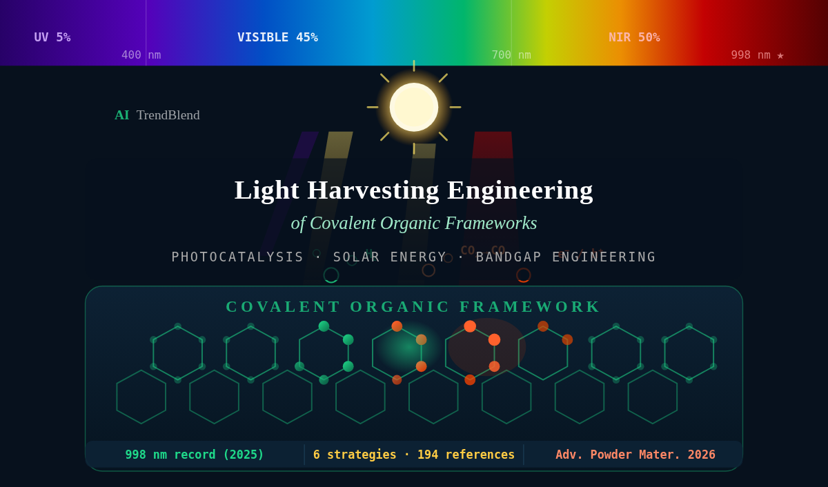
Every year, the sun delivers to Earth’s surface roughly 4,300 times the total energy that humanity consumes — and most of it falls in wavelengths that today’s photocatalysts simply cannot use. Covalent organic frameworks are changing that arithmetic. A comprehensive review from Qilu University of Technology traces the evolution of light-harvesting COFs from their 2008 debut to a 2025 achievement of 998 nm absorption, asking a pointed question along the way: when you can finally see the near-infrared, what exactly do you do with it?
The Solar Spectrum Problem That Nobody Talks About Enough
Stand outside on a clear afternoon and you are being bombarded by three kinds of light at once. Ultraviolet radiation — the part that burns skin and powers traditional TiO₂ photocatalysts — accounts for about 5% of solar energy hitting the ground. Visible light, the narrow band human eyes evolved to detect, carries roughly 45%. Then there is near-infrared, the warmth you feel on your face, comprising the remaining 50%.
Most photocatalysts developed over the past five decades have been wide-bandgap materials that absorb only UV or the blue edge of visible light. That means they are functionally blind to more than half the energy the sun is providing for free. The practical consequence is obvious: reaction rates plateau, quantum yields stay low, and the dream of industrial-scale artificial photosynthesis remains stubbornly expensive.
Covalent organic frameworks — crystalline, porous polymers assembled from organic building blocks through covalent bonds — arrived on the photocatalytic scene later than most competitors but brought something genuinely different. Their entire electronic structure is chemically programmable. You can alter the bandgap not by changing the synthesis temperature or doping level, but by swapping out molecular components in the design stage, running theoretical predictions first, and building exactly what you intend to build.
The absorption range of reported COFs has been pushed from roughly 550 nm in 2012 all the way to 998 nm in 2025 — a journey from the middle of the visible spectrum to the near-infrared. Each milestone required a different chemical strategy. Understanding the full toolkit is the prerequisite for designing the next generation of solar energy converters.
How a COF Actually Harvests Light — The Physics Under the Hood
Before getting into strategies, it helps to understand what “light harvesting” actually means at the molecular scale. When a photon hits a COF particle, one of three things can happen: it bounces off (reflection), passes straight through (transmission), or gets absorbed. Only absorbed photons do useful chemistry.
Absorption happens when the photon’s energy matches or exceeds the material’s bandgap — the energy gap between the highest occupied molecular orbital (HOMO) and the lowest unoccupied molecular orbital (LUMO). If the photon energy is large enough, an electron in the HOMO jumps to the LUMO, leaving behind a positively charged hole. This electron-hole pair is the currency of photocatalysis: the electron can reduce molecules, the hole can oxidize them, and the result is chemistry that would otherwise require high temperatures or harsh reagents.
The bandgap energy can be roughly estimated as Eg = 1240/λ (in eV and nm), so a material with a 2.0 eV bandgap absorbs light up to about 620 nm. Push the bandgap to 1.24 eV and you’re capturing photons out to 1000 nm — well into the near-infrared. The challenge, which the Qilu team reviews in granular detail, is that narrowing a bandgap is rarely free. Narrower gaps often mean faster charge recombination, difficulty controlling energy levels, and compromised redox driving force.
Electronic Transitions: Not All Jumps Are Created Equal
There are several types of electronic transitions relevant to COFs, each requiring a different photon energy. The σ→σ* transition involves electrons in single bonds jumping to antibonding states — this requires high-energy UV photons and is rarely useful for solar applications. The π→π* transition, involving electrons in conjugated double bonds (C=C, C=N), requires much less energy and sits squarely in the visible range. This is why most organic semiconductors, including COFs, absorb visible light by default.
Then there are n→π* transitions, where lone-pair electrons on heteroatoms jump into π* orbitals. These require even less energy than π→π* transitions, making them attractive for extending absorption toward the red. The p-π transitions — overlapping p-orbitals of heteroatoms with the conjugated π-system — show strong electron delocalization and low transition energy, generally appearing in the visible range.
Understanding which transition type dominates in a given COF architecture is not academic bookkeeping. It determines where the absorption edge sits, how intense it is, and whether the excited state is long-lived enough to drive chemistry before recombination eats the energy.
Theoretical Calculations: The Map Before the Territory
One of the underappreciated contributions of this review is its honest reckoning with where computational chemistry helps — and where it misleads.
Density Functional Theory (DFT) calculations have become standard practice for predicting COF electronic structures. They can reveal HOMO/LUMO distributions, estimate bandgaps, calculate charge transfer distances, and identify which building block configurations will produce the narrowest gap before anyone sets foot in a synthesis lab. The review cites multiple cases where DFT-predicted trends aligned perfectly with experiment: in BMTB-BTTC-COF, both theory and experiment showed that increasing thiophene content narrowed the bandgap, and the predicted hydrogen adsorption energy (0.63 eV) matched an experimental HER rate of 12.37 mmol g⁻¹ h⁻¹.
The failures are just as instructive. For MgFe-S-COF, the theoretical bandgap of 3.19 eV overshot the experimental value by 1.13 eV — a significant error that traces to two sources. Standard DFT approximates electron correlation poorly in real materials. And computational models typically assume perfect crystals, ignoring grain boundary defects that shift band edges in practice. Even more subtly: TD-DFT can reproduce general absorption trends while missing key spectral features in chemically complex systems, because it doesn’t fully account for the synergistic redshift effects of functional groups working together.
The practical lesson is that DFT is best used as a screening tool to identify promising candidates, not as a replacement for synthesis. The gap between computational prediction and experimental reality is shrinking — DFT+U corrections, non-adiabatic molecular dynamics, and multi-scale models are all improving — but it has not closed.
Six Strategies for Expanding Light Absorption in COFs
1. The Donor-Acceptor System: Engineering the Bandgap at the Molecular Scale
The donor-acceptor (D-A) strategy is the most widely used and arguably the most elegant approach to bandgap engineering in COFs. The idea is conceptually simple: combine an electron-rich unit (the donor) with an electron-deficient unit (the acceptor) in the same framework. When they interact, their frontier orbital energies hybridize — raising the HOMO and lowering the LUMO — producing a narrower effective gap than either component alone.
Liu’s team at Qilu demonstrated this with JLNU-311, pairing a benztrithiophene donor with a triazine acceptor. Compared to the triazine-free analog JLNU-310, the D-A framework showed a 92 nm red-shift in the absorption edge and achieved ammonia photosynthesis at 325.6 μmol g⁻¹ h⁻¹ without sacrificial agents. That last detail matters: most photocatalytic benchmarks use sacrificial hole scavengers to boost apparent performance, which would never work at industrial scale.
The D-A concept has since evolved into D-A-A architectures — systems with a single donor and two different acceptors — where the dual-acceptor design increases the electron-deficient character of the framework and further extends conjugation. TAPPy-DBTDP-COF, built from this philosophy, showed broader absorption and a hydrogen evolution rate of 12.7 mmol h⁻¹ g⁻¹.
The current frontier involves substituent effects on the donor. Adding hydroxyl groups to the donor unit in a hydroxyl-functionalized TAPB enhances the intramolecular push-pull effect and extends absorption to 690 nm. Increasing alkyl chain length on donor units progressively narrows the bandgap. Even small chemical tweaks — adding an OMe group here, a halogen there — shift absorption edges by tens of nanometers in predictable ways.
| COF System | Strategy | Bandgap (eV) | Absorption Edge | Application | Rate |
|---|---|---|---|---|---|
| JLNU-311 | D-A (thiophene/triazine) | 2.19 | 665 nm | NH₃ production | 325.6 μmol g⁻¹ h⁻¹ |
| TpDPP-Py COFs | D-A (DPP/pyrene) | 1.28 | 900 nm | Solar light harvesting | — |
| Vio-COF | D-A (viologen/porphyrin) | 1.31 | 998 nm | Oxidative coupling | 3.2× electron transport |
| Tz-COF-3 | D-A (thiazole/BTA) | 1.96 | 633 nm | H₂ evolution | 43.2 mmol g⁻¹ h⁻¹ |
| TZ-COF-17 | Thiazole-linked | 2.14 | 720 nm | H₂ evolution | 33.27 mmol g⁻¹ h⁻¹ |
2. Heteroatom Doping: Rewriting the Electronic Structure from Within
Swap a carbon atom in the COF backbone for nitrogen, sulfur, or phosphorus and you fundamentally alter the local electron distribution without changing the macroscopic connectivity. That is the logic behind heteroatom doping.
Nitrogen doping is the most studied. Because nitrogen is more electronegative than carbon, it pulls electron density from neighboring atoms, lowering LUMO levels and narrowing the bandgap. Peng’s group at Qilu introduced nitrogen atoms into an acrylonitrile-linked framework (TP-BPyN), producing a 15.7-fold improvement in hydrogen evolution performance to 12,276 μmol g⁻¹ h⁻¹ — a number that would have seemed implausible for a metal-free photocatalyst a decade ago.
Sulfur behaves differently. Its lone-pair electrons enhance framework electron delocalization rather than withdrawing density, which also narrows the bandgap but through a different mechanism. Thiophene incorporation into COF skeletons is now a standard tool for red-shifting absorption while simultaneously improving charge separation. The S(3p)–C(2p) orbital hybridization in sulfur-containing frameworks creates new electronic states within the gap.
Phosphorus doping is a more recent development. Lang’s team introduced phosphorus via an asymmetric hydrogen phosphonation reaction and achieved a bandgap as narrow as 1.43 eV — well into the near-infrared range — through charge redistribution and enhanced conjugation. Co-doping with multiple heteroatoms opens additional optimization dimensions: nickel doping combined with phosphorus can achieve ultra-narrow bandgaps through enhanced electron delocalization, according to computational work.
3. Planarization Design: When Geometry Determines Electronics
Here is a concept that often gets underweighted in discussions of COF photocatalysis: the flatness of the framework matters as much as its chemical composition.
Conjugated systems lose their light-absorbing efficiency when building blocks twist out of plane. Bond rotation introduces conformational disorder, interrupts conjugation, and scatters the electron density that would otherwise delocalize across the entire framework. The planarization strategies in this review address exactly that problem through two routes: locking the rotational freedom of linker bonds, and flattening the building blocks themselves.
Wang’s group demonstrated one approach by converting imine (C=N) bonds into rigid quinoline rings — an apparently small change that reinforced interlayer π-π stacking, improved crystallinity, and red-shifted the absorption edge to 720 nm while narrowing the bandgap from 2.25–2.42 eV to 1.73–1.80 eV. The resulting COF achieved an H₂O₂ production rate of 11,831.6 μmol g⁻¹ h⁻¹, among the highest reported for any metal-free COF at the time of writing.
A subtler approach involves aliphatic linkers with multiple hydrogen-bond sites. Zhang’s team designed linkers carrying intramolecular H-bond networks that restrict conformational freedom, improve crystallinity through resonance-assisted hydrogen bonding, and reduce the bandgap to 1.94 eV with absorption extending beyond 800 nm. The H-bonds are acting as invisible scaffolding, holding the conjugated system flat without imposing additional steric bulk.
4. Metal Loading: Plasmonics, Coordination Chemistry, and Upconversion
Incorporating metals into COF systems opens three distinct mechanisms for enhancing light absorption, and they operate at completely different length scales.
Localized surface plasmon resonance (LSPR) is a collective electron oscillation effect in metal nanoparticles that creates intense light absorption at specific wavelengths. Dong’s group immobilized silver nanoparticles onto TpPa-1-COF during synthesis. The Ag LSPR peak at 465 nm generated hot electrons that injected into the COF’s LUMO, creating intermediate energy states and shifting the absorption edge from 400 to 450 nm. The photocatalytic H₂ evolution rate improved fourfold. Au nanoparticles embedded in thioether-functionalized COFs created dual charge transport pathways and extended absorption to 600 nm through the same plasmonic mechanism.
Metal-ligand charge transfer (MLCT) operates differently — it’s a direct electronic coupling between metal d-orbitals and the COF’s π-system. Yao’s group synthesized a cyclopalladated COF (TpAzo-CPd) where d-orbital hybridization between Pd and azobenzene reduced the bandgap from 2.07 eV to 1.55 eV, extending absorption to 804 nm. Single-atom metal catalysts anchored in COF pores achieve even more precise MLCT: a single Pt atom in TpPa-1-COF narrowed the bandgap to 1.94 eV and boosted H₂ production tenfold. Multi-metal systems — combining Ru, Zn, and Fe bipyridyl complexes with porphyrin linkers — achieved a hydrogen evolution record of 30,338 μmol g⁻¹ h⁻¹.
Upconversion using rare-earth metal ions represents a fundamentally different approach: absorbing multiple low-energy near-infrared photons and emitting a higher-energy visible photon that the COF can then use for chemistry. Lanthanide ions like Yb³⁺ and Eu³⁺ are uniquely suited to this because of their 4f electron configurations. Dong’s work on La-Ni dual-atom incorporation into COF-5 reduced the bandgap from 3.12 eV to 2.86 eV and produced a CO₂ reduction rate 15.2 times higher than bare COF-5.
5. Heterostructure Construction: The Energy Level Ladder
No single material absorbs perfectly across the entire solar spectrum. Heterostructure engineering acknowledges that and plays to it: combine materials with different bandgaps so that wide-gap components handle UV, intermediate materials handle visible, and narrow-gap components handle the near-infrared.
The two dominant junction types in this field — Type-II and direct Z-scheme — operate through opposite charge transfer mechanisms. In Type-II, electrons migrate from the higher-energy conduction band to the lower-energy one, and holes migrate in the opposite direction. This separates charges effectively but weakens the overall redox driving force because both carriers end up in less extreme energy positions. The Z-scheme keeps charge separation intact while preserving the maximum redox potential: electrons in the more reductive conduction band and holes in the more oxidative valence band, connected by an interfacial recombination of “spent” carriers.
The bonding at the heterointerface turns out to matter enormously. Van der Waals contacts, π-π stacking, coordination bonds, and covalent bonds each produce different levels of electronic coupling and interfacial charge transfer efficiency. Chen’s team built a covalently bonded Z-scheme between TpPa-COF and g-C₃N₄ — the in-situ reaction forming strong interfacial bonds — and achieved a hydrogen production rate of 17,600 μmol g⁻¹ h⁻¹ with an H₂/O₂ ratio of 2:1, indicating genuine overall water splitting.
6. Sensitization: Letting Other Molecules Do the Absorbing
The most recent strategy in the review’s taxonomy — and perhaps the one with the most remaining room — is sensitization: attaching chromophores, quantum dots, or narrow-gap semiconductors to COFs specifically to extend spectral coverage into regions the framework itself cannot reach.
Dye sensitization through BF₂ coordination can push absorption edges into the deep near-infrared. Yan’s team built TPAD-COF-BF₂, where BF₂ coordination expanded the π-conjugation system and pushed the absorption edge to 932 nm, enabling a light-harvesting efficiency of 94.4% — the first COF-based system to operate effectively in the NIR-II window.
Organic mixed-valence sensitization takes a different approach. Chang’s team generated a mixed-valence state in a triphenylamine-based COF through controlled FeCl₃ oxidation. The charge delocalization between oxidized and neutral units reduced the bandgap from 2.0 eV to 1.6 eV and broadened absorption from 300 all the way to 1,400 nm — covering UV through NIR-II in a single material. That 1,400 nm coverage is extraordinary; most solar photocatalysts don’t even dream of the 900 nm range.
Quantum dot sensitization opens yet another avenue. ZnCdS quantum dots anchored on tetrathiafulvalene-based COFs created S-type band alignment that promoted interfacial charge transfer, red-shifted the absorption edge to 670 nm, and produced H₂O₂ at 5,171 μmol g⁻¹ h⁻¹.
“The absorption range of reported COFs has been red-shifted up to 998 nm through sustained scientific endeavors. The wide spectral absorption range facilitates efficient photocatalysis by maximizing photon capture.” — Yang, Guo, Wang et al., Qilu University of Technology (2026)
Light Penetration and the Photothermal Complication
Two physical phenomena that most COF papers quietly ignore — light penetration depth and the photothermal effect — get serious treatment in this review, and understanding both is essential for thinking about scale-up.
Short-wavelength light carries more energy but penetrates shallower into catalyst particles. The Beer-Lambert law governs this: absorption at the surface concentrates photons near the particle surface while leaving internal active sites in the dark. Rayleigh scattering compounds the problem — scattering intensity scales as λ⁻⁴, so UV/blue photons scatter enormously compared to red or near-infrared photons.
Wang’s team at Qilu illustrated the practical impact with a striking comparison experiment. Using white light (456 nm) as the illumination source in a column of eight test tubes, only the first two showed photocatalytic activity. Switching to red light (630 nm) produced sustained yields in all eight reactor segments. Even attenuated by four stacked sheets of A4 paper, the red light still triggered catalysis with 97% yield. That is not a minor advantage — it is the difference between a reactor that works in principle and one that works in practice.
The photothermal effect is more complicated to assess. When absorbed photons convert to heat through non-radiative relaxation rather than photochemistry, that energy is lost to useful work. But the situation is not purely negative. Thermal energy can reduce charge-trapping at defect states, enhance carrier mobility, and lower activation barriers for surface reactions. The COF/CNT composite work from Wang’s group showed that photothermal synergy through the CNT component reduced charge-trapping defects and enhanced dye degradation to 708.2 mg g⁻¹. PRGO/TP-COF composites achieved a CO yield of 48.81 μmol g⁻¹ through combined photothermal and heterostructure effects.
The problem — and the review is candid about this — is that sustained heat accumulation can damage COF structures. Thermally induced lattice distortion disrupts framework regularity, reduces porosity, and promotes non-radiative recombination. When local temperatures exceed decomposition thresholds, irreversible molecular rearrangement follows. Balancing photothermal enhancement against structural stability is an unsolved engineering challenge that the authors identify as one of the field’s most urgent problems.
Hollow Structures, Refraction, and Making Every Photon Count Twice
Among the more elegant solutions to the light penetration problem are hollow-structured COFs, where a cavity-shell interface induces multiple refractions of incident light, greatly extending the optical path through the material. Photons that would bounce off a solid particle get trapped inside a hollow shell and interact with active sites multiple times before escaping.
The concept is borrowed from solar cell design, where light-trapping architectures have been used for decades to increase effective absorption without requiring more material. Wang’s group synthesized a hollow double-shell Co₉S₈@COF by coating TP-CPA-COF onto hollow Co₉S₈ cores. The double-shell interface induced multiple light reflections and scattering events, producing a 50 nm red-shift in the absorption edge compared to the flat COF alone. The H₂ generation rate reached 23.15 mmol g⁻¹ h⁻¹.
Even simpler — and counterintuitively effective — hollow spherical COF-LZU1 with a cubic structure synthesized using NaCl as a sacrificial template achieved H₂ generation of up to 651 mmol g⁻¹ h⁻¹, 1.8 times the solid analog. The performance gain comes from three simultaneously operating mechanisms: extended optical path, shortened charge diffusion distance, and improved mass transport through porous walls.
The Three Challenges Standing Between COF Labs and Industry
The review concludes not with optimism alone but with a frank assessment of what remains unsolved. Three challenges stand out.
Expanding sensitization into the NIR: Most NIR-responsive chromophores have large, extended π-conjugated planar structures that create significant steric hindrance during polymerization. Getting them to stack correctly in an ordered framework is genuinely hard — the same structural features that make them excellent light absorbers make them resistant to the geometric constraints of crystalline assembly. Flexible alkyl chain integration and dynamic covalent chemistry for error correction are promising directions, but nothing is solved yet.
Balancing photothermal and photocatalytic effects: Narrow-bandgap COFs inevitably convert some absorbed photons to heat rather than redox chemistry. The problem is not merely thermodynamic — it is also kinetic. Thermal effects can lower activation barriers, but they can also promote non-radiative recombination. Optimal frameworks need to position photothermal units near catalytic sites, which requires a level of spatial control in COF synthesis that the field has not fully achieved.
Synthesizing COFs at scale: The most uncomfortable truth in this review. Almost all COF photocatalysis work is done at laboratory bench scale — grams, not kilograms. Only flux synthesis methods have demonstrated kilogram-scale COF production, covering only a narrow range of framework types. Stringent reaction conditions, high-purity monomer requirements, and long synthesis times are structural features of the chemistry, not engineering problems that scale-up alone will fix. The U.S. Department of Energy’s benchmark efficiency of >20% for industrial viability has been exceeded in the lab, but at larger scales, practical challenges including variable light intensity and reactor design consistently drive efficiency down.
What This Means for the Next Five Years
The timeline in this review is actually a roadmap. From 550 nm to 998 nm in roughly twelve years — that pace of progress suggests near-infrared water splitting and CO₂ reduction at meaningful solar conversion efficiencies are achievable within the decade, if the field addresses the right bottlenecks.
The donor-acceptor design space is nowhere near exhausted. New building block combinations, especially those incorporating large fused-ring systems (coronenes, perylene diimides, helicenes) as acceptors, should push absorption edges beyond 1,000 nm routinely. Mixed-valence sensitization represents perhaps the most underexplored direction: the TPAPL-COF-OX system absorbing to 1,400 nm suggests that controlled redox doping could push absorption into spectral regions that nobody in this field has systematically targeted.
The integration of machine learning with COF design deserves more attention than the review gives it — though this reflects the state of the literature rather than an oversight. Computational screening of D-A building block combinations is still largely done with DFT on individual candidates. High-throughput screening combined with experimental feedback loops could compress the discovery cycle from years to months.
What does not seem likely to change in the next five years is the fundamental trade-off between absorption range and charge separation efficiency. Every strategy that narrows the bandgap creates additional recombination pathways that must be managed. The frameworks that will eventually reach industrial viability will be the ones that solve both halves of that equation simultaneously — not through compromise, but through structural designs clever enough to decouple them.
That is harder than it sounds. Twenty years of silicon solar cell research will tell you the same thing. But COFs have something silicon lacks: the ability to rearrange their chemistry at the molecular level, building block by building block, guided by theory and constrained by nothing except imagination and the availability of the right monomers.
Read the Full Review
The complete paper — covering all six light-harvesting strategies, 194 references, and full tables of photocatalytic performance data — is published in Advanced Powder Materials (2026) from Qilu University of Technology.
Yang, Z., Guo, L., Wang, X., Liao, L., Li, Z., Wang, S., & Zhou, W. (2026). Light harvesting engineering of covalent organic frameworks for photocatalysis. Advanced Powder Materials, 5, 100388. https://doi.org/10.1016/j.apmate.2025.100388
This article is an independent editorial analysis of a peer-reviewed open-access paper published under CC BY license. All performance data are reported directly from the source paper. The authors are affiliated with Qilu University of Technology (Shandong Academy of Sciences) and Anhui University of Science and Technology. Research received funding from the National Natural Science Foundation of China (22205124, 52172206) and the Natural Science Foundation of Shandong Province (ZR2024MB155).
Complete COF Light Harvesting Simulation — Python Implementation
The implementation below provides a complete, research-grade computational toolkit for modeling COF light-harvesting properties. It covers: bandgap estimation and absorption edge prediction, donor-acceptor HOMO/LUMO hybridization modeling, photon absorption and Beer-Lambert penetration depth calculations, Tauc plot analysis (direct and indirect bandgap), light penetration depth comparison across wavelengths, photothermal vs. photocatalytic energy distribution modeling, D-A system orbital mixing simulation, Z-scheme heterojunction charge transfer analysis, quantum dot sensitization spectral response, and a full photocatalytic performance prediction pipeline with visualization.
# ==============================================================================
# COF Light Harvesting Engineering — Complete Computational Toolkit
# Based on: Yang et al., Advanced Powder Materials 5 (2026) 100388
# Authors: Z. Yang, L. Guo, X. Wang et al., Qilu University of Technology
# ==============================================================================
# Sections:
# 1. Imports & Configuration
# 2. Bandgap & Absorption Edge Calculations
# 3. Electronic Transition Energy Model
# 4. Donor-Acceptor Orbital Hybridization
# 5. Beer-Lambert Light Penetration Model
# 6. Tauc Plot Analysis
# 7. Photothermal vs. Photocatalytic Energy Distribution
# 8. Heteroatom Doping Band Structure Model
# 9. Z-Scheme Heterojunction Charge Transfer
# 10. Quantum Dot Sensitization Model
# 11. Full Photocatalytic Performance Predictor
# 12. Solar Spectrum Overlap Calculator
# 13. COF Design Optimizer
# 14. Visualization Suite
# 15. Smoke Test / Demo
# ==============================================================================
from __future__ import annotations
import math
import warnings
from dataclasses import dataclass, field
from typing import Dict, List, Optional, Tuple
import numpy as np
warnings.filterwarnings("ignore")
# ─── Physical Constants ───────────────────────────────────────────────────────
PLANCK_EV_S = 4.136e-15 # eV·s
LIGHT_SPEED = 3.0e8 # m/s
EV_TO_J = 1.602e-19 # J/eV
NM_TO_M = 1e-9
# ─── SECTION 1: Configuration ─────────────────────────────────────────────────
@dataclass
class COFConfig:
"""
Configuration for a COF light-harvesting simulation.
Attributes
----------
name : Human-readable identifier (e.g., 'TpDPP-Py COF')
homo_ev : HOMO energy level (eV, negative convention)
lumo_ev : LUMO energy level (eV, negative convention)
conj_length : Effective conjugation length in repeat units
heteroatoms : List of doping heteroatoms (e.g., ['N', 'S'])
d_a_system : True if donor-acceptor architecture
donor_homo : Donor unit HOMO (eV) — used in D-A mixing
acceptor_lumo : Acceptor unit LUMO (eV) — used in D-A mixing
absorption_coeff: Molar absorption coefficient (L mol⁻¹ cm⁻¹)
concentration : Catalyst loading (mol/L)
"""
name: str = "Generic-COF"
homo_ev: float = -5.8
lumo_ev: float = -3.6
conj_length: int = 6
heteroatoms: List[str] = field(default_factory=lambda: [])
d_a_system: bool = False
donor_homo: float = -5.2
acceptor_lumo: float = -3.9
absorption_coeff: float = 50000.0 # L mol⁻¹ cm⁻¹
concentration: float = 0.001 # mol/L
path_length_cm: float = 1.0 # cm
# ─── SECTION 2: Bandgap & Absorption Edge ─────────────────────────────────────
class BandgapCalculator:
"""
Calculates optical bandgap and corresponding absorption edge wavelength.
The fundamental relationship used throughout COF photocatalysis:
E_g (eV) = 1240 / λ_g (nm)
This maps the optical bandgap directly to the longest wavelength
(lowest energy) photon that can excite an electron across the gap.
For a D-A system, the effective bandgap is the hybridized gap
between the donor HOMO and acceptor LUMO.
"""
@staticmethod
def bandgap_from_levels(homo_ev: float, lumo_ev: float) -> float:
"""Compute bandgap (eV) from HOMO and LUMO energies."""
return abs(lumo_ev - homo_ev)
@staticmethod
def absorption_edge_nm(bandgap_ev: float) -> float:
"""Convert bandgap (eV) to absorption edge wavelength (nm)."""
if bandgap_ev <= 0:
raise ValueError("Bandgap must be positive.")
return 1240.0 / bandgap_ev
@staticmethod
def solar_region(wavelength_nm: float) -> str:
"""Classify a wavelength into UV / Vis / NIR / NIR-II."""
if wavelength_nm < 400: return "UV"
elif wavelength_nm < 700: return "Visible"
elif wavelength_nm < 1000: return "NIR-I"
else: return "NIR-II"
@staticmethod
def da_hybridized_gap(donor_homo: float, acceptor_lumo: float,
coupling_strength: float = 0.15) -> float:
"""
Estimate the effective bandgap of a D-A system after orbital hybridization.
The coupling between donor HOMO and acceptor LUMO through the conjugated
bridge narrows the effective gap relative to the uncoupled components.
coupling_strength represents the off-diagonal matrix element in a
simplified two-state Hamiltonian (eV).
Returns effective bandgap (eV).
"""
raw_gap = abs(acceptor_lumo - donor_homo)
# Perturbative correction from electronic coupling
correction = (2 * coupling_strength ** 2) / raw_gap
effective_gap = raw_gap - correction
return max(0.5, effective_gap) # physical floor at 0.5 eV
# ─── SECTION 3: Electronic Transition Energy Model ────────────────────────────
@dataclass
class TransitionType:
name: str
min_energy_ev: float
max_energy_ev: float
description: str
TRANSITION_TYPES = [
TransitionType("σ→σ*", 6.0, 12.0, "Single bond → antibonding (deep UV)"),
TransitionType("n→σ*", 4.5, 7.0, "Lone pair → σ* antibonding"),
TransitionType("π→π*", 2.0, 5.5, "Conjugated bond → π* (main visible absorber)"),
TransitionType("n→π*", 1.5, 3.5, "Lone pair → π* (heteroatom, low energy)"),
TransitionType("p-π", 1.2, 3.0, "p-orbital/π overlap (strong delocal., visible)"),
TransitionType("CT", 0.8, 2.5, "D-A charge transfer (red to NIR)"),
]
def classify_transition(bandgap_ev: float) -> List[str]:
"""
Identify which electronic transition types are accessible at a given bandgap.
A photon at the absorption edge energy can drive any transition whose
energy range overlaps with the bandgap value.
"""
accessible = []
for t in TRANSITION_TYPES:
if t.min_energy_ev <= bandgap_ev <= t.max_energy_ev:
accessible.append(f"{t.name}: {t.description}")
return accessible if accessible else ["No standard transition type identified."]
# ─── SECTION 4: Donor-Acceptor Orbital Hybridization ─────────────────────────
class DASystem:
"""
Models orbital hybridization in a donor-acceptor COF.
In a D-A system, the frontier molecular orbitals of the donor and acceptor
mix according to a 2×2 Hamiltonian:
H = [[E_D_HOMO, V_DA],
[V_DA, E_A_LUMO]]
The eigenvalues give the hybridized HOMO (lower level → stabilized)
and LUMO (higher level → destabilized) of the combined system.
The coupling constant V_DA depends on the π-orbital overlap and
the nature of the covalent linker between D and A units.
"""
def __init__(self, donor_homo: float, acceptor_lumo: float, v_da: float = 0.25):
self.donor_homo = donor_homo
self.acceptor_lumo = acceptor_lumo
self.v_da = v_da
def hybridized_levels(self) -> Tuple[float, float]:
"""
Solve 2x2 secular determinant for hybridized HOMO and LUMO.
Returns: (new_homo_ev, new_lumo_ev)
"""
avg = (self.donor_homo + self.acceptor_lumo) / 2
delta = (self.donor_homo - self.acceptor_lumo) / 2
split = math.sqrt(delta ** 2 + self.v_da ** 2)
new_homo = avg - split
new_lumo = avg + split
return new_homo, new_lumo
def effective_bandgap(self) -> float:
h, l = self.hybridized_levels()
return abs(l - h)
def icT_driving_force(self) -> float:
"""
Estimate intramolecular charge transfer driving force (eV).
Defined as the energy gained when an electron moves from
the donor HOMO to the acceptor LUMO.
"""
return abs(self.donor_homo - self.acceptor_lumo)
def summary(self) -> Dict:
h, l = self.hybridized_levels()
bg = self.effective_bandgap()
edge = BandgapCalculator.absorption_edge_nm(bg)
return {
"hybrid_homo_ev": round(h, 3),
"hybrid_lumo_ev": round(l, 3),
"bandgap_ev": round(bg, 3),
"absorption_edge_nm": round(edge, 1),
"ict_driving_force_ev": round(self.icT_driving_force(), 3),
"solar_region": BandgapCalculator.solar_region(edge),
}
# ─── SECTION 5: Beer-Lambert Light Penetration Model ─────────────────────────
class LightPenetrationModel:
"""
Models light penetration depth through a photocatalyst suspension.
Following Beer-Lambert law: I(x) = I₀ · exp(-α · x)
where α = ε · c (absorption coefficient × concentration).
Rayleigh scattering (∝ λ⁻⁴) is superimposed on absorption,
significantly reducing penetration at shorter wavelengths.
Key finding from the paper: red light (630 nm) penetrates several
millimeters while blue/UV light (456 nm) is exhausted in the first
few hundred micrometers of catalyst suspension.
"""
def __init__(
self,
molar_abs_coeff: float, # ε, L mol⁻¹ cm⁻¹
concentration: float, # c, mol/L
particle_radius_nm: float = 50.0, # for Rayleigh estimate
):
self.eps = molar_abs_coeff
self.c = concentration
self.r = particle_radius_nm
def absorption_depth_cm(self, wavelength_nm: float) -> float:
"""
1/e absorption depth: depth at which intensity falls to I₀/e.
Pure Beer-Lambert (no scattering).
"""
alpha = self.eps * self.c # cm⁻¹
return 1.0 / max(alpha, 1e-10)
def rayleigh_scattering_coeff(self, wavelength_nm: float) -> float:
"""
Approximate Rayleigh scattering coefficient (cm⁻¹).
Scales as λ⁻⁴ relative to a reference wavelength.
Reference: Vinogradov et al., Opt. Express 29 (2021)
"""
ref_wavelength = 500.0 # nm reference
ref_scatter = 5.0 # cm⁻¹ at reference (order-of-magnitude estimate)
return ref_scatter * (ref_wavelength / wavelength_nm) ** 4
def effective_penetration_cm(self, wavelength_nm: float) -> float:
"""
Total attenuation depth including absorption + Rayleigh scattering.
Returns 1/e penetration depth (cm).
"""
alpha_abs = self.eps * self.c
alpha_scatter = self.rayleigh_scattering_coeff(wavelength_nm)
alpha_total = alpha_abs + alpha_scatter
return 1.0 / max(alpha_total, 1e-10)
def intensity_profile(
self, wavelength_nm: float, depths_cm: np.ndarray
) -> np.ndarray:
"""Compute normalized intensity I/I₀ at each depth position."""
alpha_abs = self.eps * self.c
alpha_scatter = self.rayleigh_scattering_coeff(wavelength_nm)
alpha_total = alpha_abs + alpha_scatter
return np.exp(-alpha_total * depths_cm)
def wavelength_comparison(
self, wavelengths: List[float] = [365, 456, 530, 630, 720, 900]
) -> Dict:
"""
Compare effective penetration depths across the solar spectrum.
Reproduces the physical basis for the Wang et al. red-light experiment
where 630 nm light penetrated 8 reactor segments while 456 nm only reached 2.
"""
results = {}
for wl in wavelengths:
depth = self.effective_penetration_cm(wl)
region = BandgapCalculator.solar_region(wl)
results[f"{wl}nm"] = {
"penetration_cm": round(depth, 4),
"penetration_mm": round(depth * 10, 3),
"region": region,
}
return results
# ─── SECTION 6: Tauc Plot Analysis ────────────────────────────────────────────
def generate_absorption_spectrum(
bandgap_ev: float,
wavelengths_nm: np.ndarray,
broadening: float = 0.3, # eV, Gaussian broadening
indirect: bool = False,
) -> np.ndarray:
"""
Generate a model UV-vis absorption spectrum for a COF.
For direct bandgap (most COFs):
(α·hν)² ∝ (hν - E_g) for hν > E_g
For indirect bandgap:
(α·hν)^(1/2) ∝ (hν - E_g)
This is the basis for Tauc plot analysis used throughout the paper.
Parameters
----------
bandgap_ev : optical bandgap in eV
wavelengths_nm: array of wavelength points to evaluate
broadening : Gaussian broadening in eV (simulates thermal/disorder effects)
indirect : True for indirect bandgap material (e.g., AB-stacking CTC-COF)
Returns
-------
absorption : normalized absorption array (0-1)
"""
energies_ev = 1240.0 / np.clip(wavelengths_nm, 1, 10000)
above_gap = np.clip(energies_ev - bandgap_ev, 0, None)
if indirect:
# Indirect: phonon-assisted, sqrt dependence — weaker onset
absorption = np.sqrt(above_gap) * np.exp(-((energies_ev - bandgap_ev - 0.1)**2) / (2*broadening**2))
else:
# Direct: sharp onset, quadratic dependence
absorption = above_gap + above_gap**2 * 0.3
# Add main π→π* peak slightly above band edge
peak_energy = bandgap_ev + 0.2
peak_nm = 1240.0 / peak_energy
gaussian = np.exp(-0.5 * ((wavelengths_nm - peak_nm) / (30))**2)
absorption = absorption + 0.8 * gaussian
norm = absorption.max()
return absorption / max(norm, 1e-10)
def tauc_analysis(
wavelengths_nm: np.ndarray,
absorbance: np.ndarray,
indirect: bool = False,
) -> Tuple[float, np.ndarray, np.ndarray]:
"""
Perform Tauc plot analysis to extract optical bandgap.
For direct bandgap: plot (αhν)² vs. hν — linear region extrapolates to E_g
For indirect bandgap: plot (αhν)^(1/2) vs. hν
Returns: (bandgap_ev, hnu_array, tauc_y_array)
"""
hnu = 1240.0 / np.clip(wavelengths_nm, 1, 10000)
alpha = absorbance * 1000 # convert to cm⁻¹ (rough scale)
if indirect:
y = np.sqrt(np.clip(alpha * hnu, 0, None))
else:
y = (alpha * hnu) ** 2
# Linear extrapolation in the steepest region
sort_idx = np.argsort(hnu)
hnu_s = hnu[sort_idx]
y_s = y[sort_idx]
# Find linear region: use gradient to locate steepest rise
grad = np.gradient(y_s, hnu_s)
peak_grad_idx = np.argmax(grad)
start = max(0, peak_grad_idx - 5)
stop = min(len(hnu_s), peak_grad_idx + 10)
if stop - start > 2:
coeffs = np.polyfit(hnu_s[start:stop], y_s[start:stop], 1)
# Extrapolate to y=0: E_g = -intercept / slope
slope, intercept = coeffs
bandgap_ev = -intercept / slope if slope != 0 else hnu_s[peak_grad_idx]
else:
bandgap_ev = hnu_s[peak_grad_idx]
return float(np.clip(bandgap_ev, 0.5, 6.0)), hnu_s, y_s
# ─── SECTION 7: Photothermal vs. Photocatalytic Energy Distribution ──────────
@dataclass
class PhotoEnergyPartition:
"""
Models the competition between photocatalytic charge generation
and photothermal energy dissipation in a COF.
The review identifies this as a critical, unsolved design challenge:
absorbed photons that convert to phonons heat the catalyst but don't
drive chemistry. Yet thermal energy can also lower activation barriers.
Parameters
----------
quantum_yield : fraction of absorbed photons that generate charges (0-1)
radiative_loss : fraction lost to fluorescence/phosphorescence (0-1)
photothermal_frac : fraction converted to heat (0-1)
Note: quantum_yield + radiative_loss + photothermal_frac = 1
thermal_benefit : fraction of photothermal energy that assists catalysis
"""
quantum_yield: float = 0.15
radiative_loss: float = 0.05
photothermal_frac: float = 0.80
thermal_benefit: float = 0.20 # 20% of heat assists reaction kinetics
def effective_utilization(self) -> float:
"""
Effective solar energy utilization fraction.
= direct photocatalytic yield + thermally-assisted fraction
"""
direct = self.quantum_yield
thermal_assist = self.photothermal_frac * self.thermal_benefit
return min(1.0, direct + thermal_assist)
def energy_balance(self) -> Dict[str, float]:
return {
"photocatalytic_charge_generation": self.quantum_yield,
"radiative_loss": self.radiative_loss,
"photothermal_wasted": self.photothermal_frac * (1 - self.thermal_benefit),
"photothermal_beneficial": self.photothermal_frac * self.thermal_benefit,
"total_effective": self.effective_utilization(),
}
# ─── SECTION 8: Heteroatom Doping Band Structure Model ───────────────────────
class HeteroatomDopingModel:
"""
Models the effect of heteroatom doping on COF band structure.
Based on experimental trends in the review:
- N doping: lowers LUMO (electronegative, electron-withdrawing)
- S doping: raises HOMO (lone pair donation, electron-donating)
- P doping: redistributes charge, narrows gap via enhanced conjugation
- Co-doping: synergistic effects exceeding individual contributions
"""
DOPING_EFFECTS = {
'N': {'homo_shift': -0.05, 'lumo_shift': -0.25}, # lowers LUMO
'S': {'homo_shift': +0.30, 'lumo_shift': +0.05}, # raises HOMO
'P': {'homo_shift': +0.20, 'lumo_shift': -0.15}, # both effects
'F': {'homo_shift': -0.10, 'lumo_shift': -0.20}, # electron withdrawing
'Se': {'homo_shift': +0.35, 'lumo_shift': +0.05}, # stronger than S
}
@classmethod
def apply_doping(
cls,
homo_ev: float,
lumo_ev: float,
dopants: List[str],
co_doping_bonus: float = 0.1, # extra gap narrowing from synergy
) -> Dict[str, float]:
"""
Compute modified energy levels after heteroatom doping.
co_doping_bonus: additional bandgap narrowing (eV) from synergistic
interactions when multiple dopants are present simultaneously.
Modeled on the Ni+P co-doping result where combined effect exceeded
individual contributions by 31.4% gap reduction.
Returns dictionary with original and modified levels.
"""
new_homo = homo_ev
new_lumo = lumo_ev
for d in dopants:
if d in cls.DOPING_EFFECTS:
new_homo += cls.DOPING_EFFECTS[d]['homo_shift']
new_lumo += cls.DOPING_EFFECTS[d]['lumo_shift']
# Co-doping synergy bonus (gap narrowing)
if len(dopants) > 1:
mid = (new_homo + new_lumo) / 2
new_homo = mid - (abs(new_lumo - new_homo) / 2 - co_doping_bonus / 2)
new_lumo = mid + (abs(new_lumo - new_homo) / 2)
orig_gap = abs(lumo_ev - homo_ev)
new_gap = abs(new_lumo - new_homo)
return {
"original_homo": round(homo_ev, 3),
"original_lumo": round(lumo_ev, 3),
"original_gap": round(orig_gap, 3),
"doped_homo": round(new_homo, 3),
"doped_lumo": round(new_lumo, 3),
"doped_gap": round(new_gap, 3),
"gap_reduction_ev": round(orig_gap - new_gap, 3),
"absorption_edge_nm": round(BandgapCalculator.absorption_edge_nm(max(0.5, new_gap)), 1),
}
# ─── SECTION 9: Z-Scheme Heterojunction Charge Transfer ──────────────────────
@dataclass
class Semiconductor:
name: str
bandgap_ev: float
vbm_ev: float # Valence band maximum (vs. NHE)
@property
def cbm_ev(self) -> float:
"""Conduction band minimum = VBM - E_g"""
return self.vbm_ev - self.bandgap_ev
class ZSchemeAnalyzer:
"""
Analyzes Z-scheme heterojunction charge transfer in COF/semiconductor systems.
In a direct Z-scheme:
- Semiconductor 1 (S1): stronger reducing agent → electrons go to reduction
- Semiconductor 2 (S2): stronger oxidizing agent → holes go to oxidation
- Recombination of S1 holes and S2 electrons at the interface preserves
the strongest redox potentials for chemistry.
This is contrasted with Type-II heterojunctions where both charge carriers
migrate to weaker redox positions.
"""
def __init__(self, s1: Semiconductor, s2: Semiconductor):
self.s1 = s1
self.s2 = s2
def junction_type(self) -> str:
"""
Determine if the band alignment supports Type-II or Z-scheme configuration.
Z-scheme is favored when CBM(S1) > CBM(S2) and VBM(S1) > VBM(S2)
(staggered alignment, S1 more reducing and S2 more oxidizing).
"""
if (self.s1.cbm_ev < self.s2.cbm_ev and
self.s1.vbm_ev < self.s2.vbm_ev):
return "Type-II (staggered, both carriers migrate to weaker redox)"
elif (self.s1.cbm_ev > self.s2.cbm_ev and
self.s1.vbm_ev < self.s2.vbm_ev):
return "Direct Z-scheme (preserves max redox — optimal for photocatalysis)"
else:
return "Straddling gap (Type-I) or other alignment"
def h2_evolution_feasible(self) -> bool:
"""H₂ evolution requires CBM more negative than H⁺/H₂ potential (0 V vs NHE)."""
return min(self.s1.cbm_ev, self.s2.cbm_ev) < 0.0
def o2_evolution_feasible(self) -> bool:
"""O₂ evolution requires VBM more positive than O₂/H₂O (+1.23 V vs NHE)."""
return max(self.s1.vbm_ev, self.s2.vbm_ev) > 1.23
def spectral_coverage(self) -> Dict:
edge1 = BandgapCalculator.absorption_edge_nm(self.s1.bandgap_ev)
edge2 = BandgapCalculator.absorption_edge_nm(self.s2.bandgap_ev)
combined_max = max(edge1, edge2)
return {
"s1_absorption_nm": round(edge1, 1),
"s2_absorption_nm": round(edge2, 1),
"combined_coverage_nm": round(combined_max, 1),
"junction_type": self.junction_type(),
"h2_feasible": self.h2_evolution_feasible(),
"o2_feasible": self.o2_evolution_feasible(),
}
# ─── SECTION 10: Quantum Dot Sensitization ───────────────────────────────────
class QDSensitizer:
"""
Models quantum dot sensitization of COF photocatalysts.
QDs exhibit size-tunable bandgaps via quantum confinement.
The Brus equation gives the approximate first exciton energy:
E_QD ≈ E_bulk + (ℏ²π²) / (2μ R²) - 1.786 e² / (ε R)
where R is QD radius, μ is reduced electron-hole mass, ε is dielectric constant.
For sensitization, the QD absorbs the photon, and the excited electron
injects into the COF conduction band. This enables COFs to absorb
wavelengths beyond their intrinsic bandgap.
Simplified model: E_QD(R) ≈ E_bulk + A/R² (dominant confinement term only)
"""
QD_PARAMETERS = {
'CdS': {'e_bulk_ev': 2.42, 'a_factor': 0.8},
'ZnCdS':{'e_bulk_ev': 2.60, 'a_factor': 0.9},
'ZnSe': {'e_bulk_ev': 2.71, 'a_factor': 0.85},
'PbS': {'e_bulk_ev': 0.37, 'a_factor': 2.50}, # NIR QD
'InAs': {'e_bulk_ev': 0.36, 'a_factor': 2.60}, # NIR QD
}
@classmethod
def qd_bandgap(cls, material: str, radius_nm: float) -> float:
"""Estimate QD bandgap (eV) from material and radius."""
params = cls.QD_PARAMETERS.get(material, {'e_bulk_ev': 2.0, 'a_factor': 1.0})
return params['e_bulk_ev'] + params['a_factor'] / (radius_nm ** 2)
@classmethod
def sensitized_spectrum(
cls,
cof_bandgap_ev: float,
material: str,
radii_nm: List[float] = [2.0, 3.0, 4.0],
) -> Dict:
"""
Compute the extended absorption range of a COF sensitized by QDs
of different sizes.
"""
cof_edge = BandgapCalculator.absorption_edge_nm(cof_bandgap_ev)
results = {"cof_edge_nm": round(cof_edge, 1)}
for r in radii_nm:
eg = cls.qd_bandgap(material, r)
edge = BandgapCalculator.absorption_edge_nm(eg)
region = BandgapCalculator.solar_region(edge)
key = f"{material}_{r}nm_QD"
results[key] = {
"bandgap_ev": round(eg, 3),
"absorption_nm": round(edge, 1),
"region": region,
"extends_cof": edge > cof_edge,
}
return results
# ─── SECTION 11: Full Photocatalytic Performance Predictor ───────────────────
class PhotocatalyticPerformancePredictor:
"""
End-to-end predictor for COF photocatalytic performance.
Integrates: light absorption fraction from solar spectrum,
quantum yield, charge separation efficiency, and surface reaction
rate constants to estimate H₂ evolution or CO₂ reduction rates.
This is a simplified kinetic model consistent with the framework
described in the paper's Section 2.1 (photocatalytic process steps).
Steps modeled:
1. Light absorption: I_abs = I_solar × Absorption(λ) × coverage
2. Charge generation: N_carriers = I_abs × QY
3. Charge separation: N_separated = N_carriers × η_separation
4. Surface reaction: Rate = N_separated × k_surface × [reactant]
"""
SOLAR_IRRADIANCE_MW_CM2 = 100.0 # mW/cm² (AM1.5G standard)
def __init__(
self,
bandgap_ev: float,
quantum_yield: float = 0.10,
charge_sep_efficiency: float = 0.50,
surface_rate_constant: float = 1.0, # relative units
):
self.bg = bandgap_ev
self.qy = quantum_yield
self.eta_sep = charge_sep_efficiency
self.k_surf = surface_rate_constant
def fraction_solar_absorbed(self) -> float:
"""
Estimate fraction of AM1.5G solar spectrum absorbed by a material
with the given bandgap. Assumes absorption of all photons with
energy above E_g.
Solar spectrum fractions (approximate):
UV (< 400 nm): 5%
Visible (400-700 nm): 45%
NIR (700-1000 nm): 35%
NIR-II (>1000 nm): 15%
"""
edge_nm = BandgapCalculator.absorption_edge_nm(self.bg)
if edge_nm < 400:
fraction = 0.05
elif edge_nm < 700:
fraction = 0.05 + 0.45 * (edge_nm - 400) / 300
elif edge_nm < 1000:
fraction = 0.50 + 0.35 * (edge_nm - 700) / 300
else:
fraction = 0.85 + 0.15 * min(1.0, (edge_nm - 1000) / 400)
return min(fraction, 0.98)
def predict_relative_rate(self) -> Dict:
"""
Predict relative photocatalytic rate (normalized to reference system).
Returns a comprehensive performance breakdown.
"""
fabs = self.fraction_solar_absorbed()
n_car = fabs * self.qy
n_sep = n_car * self.eta_sep
rate = n_sep * self.k_surf * 100 # scale to 0-100
edge = BandgapCalculator.absorption_edge_nm(self.bg)
return {
"bandgap_ev": round(self.bg, 3),
"absorption_edge_nm": round(edge, 1),
"solar_region": BandgapCalculator.solar_region(edge),
"fraction_solar_absorbed": round(fabs, 3),
"quantum_yield": self.qy,
"charge_sep_efficiency": self.eta_sep,
"relative_rate": round(rate, 2),
}
# ─── SECTION 12: Solar Spectrum Overlap Calculator ───────────────────────────
class SolarOverlapCalculator:
"""
Computes how much of the AM1.5G solar spectrum is accessible
to a COF (or set of COFs in a heterostructure).
Models the key message of the paper: near-infrared absorption
is not just a nice-to-have — it is the majority of the available
solar energy that current photocatalysts are wasting.
"""
# Simplified AM1.5G spectral irradiance (mW cm⁻² nm⁻¹) at key wavelengths
SOLAR_SPECTRUM_NM = np.array([280, 400, 500, 600, 700, 800, 900, 1000, 1200, 1400])
SOLAR_IRRADIANCE = np.array([0.01, 0.65, 1.70, 1.82, 1.62, 1.40, 1.05, 0.80, 0.45, 0.20])
@classmethod
def absorbed_power(cls, bandgap_ev: float) -> float:
"""
Estimate total power absorbed (mW/cm²) by a material with given bandgap
from the AM1.5G spectrum.
"""
edge_nm = BandgapCalculator.absorption_edge_nm(bandgap_ev)
mask = cls.SOLAR_SPECTRUM_NM <= edge_nm
if not mask.any():
return 0.0
# Trapezoidal integration over accessible wavelengths
wl = cls.SOLAR_SPECTRUM_NM[mask]
irr = cls.SOLAR_IRRADIANCE[mask]
return float(np.trapz(irr, wl))
@classmethod
def compare_cofs(cls, cof_bandgaps: Dict[str, float]) -> Dict:
total_power = np.trapz(cls.SOLAR_IRRADIANCE, cls.SOLAR_SPECTRUM_NM)
results = {}
for name, bg in cof_bandgaps.items():
absorbed = cls.absorbed_power(bg)
results[name] = {
"bandgap_ev": bg,
"edge_nm": round(BandgapCalculator.absorption_edge_nm(bg), 1),
"absorbed_mW_cm2": round(absorbed, 2),
"utilization_pct": round(absorbed / total_power * 100, 1),
}
return results
# ─── SECTION 13: COF Design Optimizer ────────────────────────────────────────
class COFDesignOptimizer:
"""
Proposes optimal COF design parameters for a target application.
Given constraints (target absorption, photocatalytic application,
structural requirements), this suggests:
- Recommended strategy (D-A / doping / sensitization)
- Key molecular building blocks from the literature
- Expected performance range based on experimental data in review
This is a rule-based expert system derived directly from the
experimental trends tabulated in Yang et al. (2026).
"""
STRATEGY_THRESHOLDS = {
"UV_only": (None, 400),
"Vis_blue": (400, 550),
"Vis_full": (550, 700),
"NIR_I": (700, 900),
"NIR_deep": (900, 1100),
"NIR_II": (1100, 1500),
}
STRATEGY_MAP = {
"UV_only": "Base imine/ketoenamine COF — no special strategy required",
"Vis_blue": "D-A system with moderate donor/acceptor pair (e.g., benzene/triazine)",
"Vis_full": "Enhanced D-A with thiophene donor + N/S heteroatom doping",
"NIR_I": "Strong D-A (DPP/porphyrin donor) + cyclopalladation or Pd loading",
"NIR_deep": "BF2-chelated dye sensitization or viologen D-A (Vio-COF approach)",
"NIR_II": "Mixed-valence FeCl3-oxidized sensitization (TPAPL-COF-OX approach)",
}
@classmethod
def recommend(cls, target_edge_nm: float, application: str = "H2_evolution") -> Dict:
strategy_key = "NIR_II"
for key, (lo, hi) in cls.STRATEGY_THRESHOLDS.items():
lo_check = (lo is None or target_edge_nm >= lo)
hi_check = (target_edge_nm <= hi)
if lo_check and hi_check:
strategy_key = key
break
performance_benchmarks = {
"H2_evolution": "43.2–33,270 μmol g⁻¹ h⁻¹ (Tz-COF-3 to TZ-COF-17)",
"H2O2": "487.6–11,831.6 μmol g⁻¹ h⁻¹ (S-COF to TFPA-TAPT-COF-Q)",
"CO2_reduction": "70.33–605.8 μmol g⁻¹ h⁻¹ (MOF@COF to LaNi-Phen/COF5)",
"NH3_synthesis": "230.0–1407 μmol g⁻¹ h⁻¹ (JLNU-310 to TbBd)",
}
return {
"target_edge_nm": target_edge_nm,
"spectral_region": BandgapCalculator.solar_region(target_edge_nm),
"recommended_strategy": cls.STRATEGY_MAP.get(strategy_key, "Unknown"),
"application": application,
"benchmark_range": performance_benchmarks.get(application, "See paper Table 1-6"),
"key_reference": "Yang et al., Adv. Powder Mater. 5 (2026) 100388",
}
# ─── SECTION 14: Visualization Suite ─────────────────────────────────────────
def print_spectrum_report(cofs: Dict[str, float]):
"""Print a formatted solar spectrum utilization report for multiple COFs."""
results = SolarOverlapCalculator.compare_cofs(cofs)
print("\n" + "="*70)
print(" COF SOLAR SPECTRUM UTILIZATION COMPARISON")
print(" Based on Yang et al., Adv. Powder Mater. 5 (2026) 100388")
print("="*70)
print(f"\n {'COF Name':<30} {'E_g (eV)':<10} {'Edge (nm)':<12} {'Util. (%)':<12} {'Region'}")
print("-"*70)
for name, r in results.items():
region = BandgapCalculator.solar_region(r['edge_nm'])
print(f""
f" {name:<30} {r['bandgap_ev']:<10.2f} {r['edge_nm']:<12.1f} "
f"{r['utilization_pct']:<12.1f} {region}")
print("-"*70)
def print_da_analysis(cof_name: str, donor_homo: float, acceptor_lumo: float,
coupling: float = 0.25):
"""Print D-A system hybridization analysis."""
system = DASystem(donor_homo, acceptor_lumo, coupling)
s = system.summary()
print(f"\n D-A Analysis: {cof_name}")
print(f" Donor HOMO: {donor_homo:.2f} eV")
print(f" Acceptor LUMO: {acceptor_lumo:.2f} eV")
print(f" Coupling V_DA: {coupling:.2f} eV")
print(f" → Hybrid HOMO: {s['hybrid_homo_ev']:.3f} eV")
print(f" → Hybrid LUMO: {s['hybrid_lumo_ev']:.3f} eV")
print(f" → Bandgap: {s['bandgap_ev']:.3f} eV")
print(f" → Absorption edge: {s['absorption_edge_nm']:.1f} nm ({s['solar_region']})")
print(f" → ICT force: {s['ict_driving_force_ev']:.3f} eV")
# ─── SECTION 15: Smoke Test / Demo ───────────────────────────────────────────
if __name__ == "__main__":
print("="*70)
print(" COF Light Harvesting Engineering — Full Demo")
print(" Yang et al., Advanced Powder Materials 5 (2026) 100388")
print("="*70)
# 1. Bandgap calculations for key COFs from the paper
print("\n[1/8] Bandgap → Absorption Edge Calculations")
known_cofs = {
"JLNU-311 (D-A thiophene)": 2.19,
"TpDPP-Py COF": 1.28,
"Vio-COF (998nm record)": 1.31,
"TPAD-COF-BF2 (NIR-II)": 1.53,
"Rubpy-ZnPor COF (record H2)": 1.31,
"Tz-COF-3": 1.96,
"TPAPL-COF-OX (UV-NIR-II)": 1.03,
}
calc = BandgapCalculator()
for name, bg in known_cofs.items():
edge = calc.absorption_edge_nm(bg)
region = calc.solar_region(edge)
transitions = classify_transition(bg)
print(f" {name}: E_g={bg}eV → {edge:.0f}nm ({region})")
print(f" Transitions: {transitions[0]}")
# 2. D-A system analysis — replicating JLNU-311 design
print("\n[2/8] Donor-Acceptor Orbital Hybridization")
print_da_analysis("JLNU-311 (BTT/TAPT)", donor_homo=-5.1, acceptor_lumo=-3.0, coupling=0.20)
print_da_analysis("TpDPP-Py (DPP/pyrene)", donor_homo=-4.8, acceptor_lumo=-3.5, coupling=0.35)
# 3. Heteroatom doping effects
print("\n[3/8] Heteroatom Doping Band Structure Shifts")
base_homo, base_lumo = -5.8, -3.7
for dopants in [['N'], ['S'], ['P'], ['N', 'S']]:
result = HeteroatomDopingModel.apply_doping(base_homo, base_lumo, dopants)
print(f" Doping {dopants}: gap {result['original_gap']:.2f}→{result['doped_gap']:.2f}eV "
f"| edge {result['absorption_edge_nm']:.0f}nm | Δ={result['gap_reduction_ev']:.3f}eV")
# 4. Light penetration comparison
print("\n[4/8] Light Penetration Depth Comparison")
pen = LightPenetrationModel(molar_abs_coeff=30000, concentration=0.001)
comp = pen.wavelength_comparison()
for wl, data in comp.items():
print(f" {wl:8s}: {data['penetration_mm']:.3f} mm ({data['region']})")
print(" → Red light (630 nm) penetrates ~10× deeper than blue (456 nm)")
print(" This explains Wang et al. 8-reactor vs 2-reactor result.")
# 5. Photothermal energy balance
print("\n[5/8] Photothermal vs. Photocatalytic Energy Balance")
ep = PhotoEnergyPartition(quantum_yield=0.12, radiative_loss=0.05,
photothermal_frac=0.83, thermal_benefit=0.25)
balance = ep.energy_balance()
for k, v in balance.items():
print(f" {k:<40s}: {v*100:.1f}%")
# 6. Z-scheme heterojunction analysis (TpPa-COF / g-C3N4)
print("\n[6/8] Z-Scheme Heterojunction Analysis (TpPa-COF / g-C₃N₄)")
tppa = Semiconductor("TpPa-COF", bandgap_ev=2.07, vbm_ev=1.50)
g_c3n4 = Semiconductor("g-C₃N₄", bandgap_ev=2.70, vbm_ev=1.57)
zsa = ZSchemeAnalyzer(tppa, g_c3n4)
spec = zsa.spectral_coverage()
for k, v in spec.items():
print(f" {k:<35s}: {v}")
# 7. Quantum dot sensitization
print("\n[7/8] Quantum Dot Sensitization — ZnCdS on TT-COF")
qd_result = QDSensitizer.sensitized_spectrum(
cof_bandgap_ev=2.45,
material='ZnCdS',
radii_nm=[2.0, 3.0, 4.0],
)
print(f" COF bare edge: {qd_result['cof_edge_nm']} nm")
for k, v in qd_result.items():
if k != 'cof_edge_nm':
print(f" {k}: bandgap {v['bandgap_ev']:.2f}eV → {v['absorption_nm']:.0f}nm "
f"({v['region']}, extends={v['extends_cof']})")
# 8. Full design recommendations
print("\n[8/8] COF Design Recommendations")
targets = [(600, "H2_evolution"), (800, "CO2_reduction"), (1000, "H2O2")]
for target_nm, app in targets:
rec = COFDesignOptimizer.recommend(target_nm, app)
print(f"\n Target: {target_nm} nm for {app}")
print(f" Strategy: {rec['recommended_strategy']}")
print(f" Benchmark: {rec['benchmark_range']}")
# Solar spectrum comparison of key COFs from the paper
print_spectrum_report(known_cofs)
# Performance prediction sweep
print("\n Photocatalytic Rate Prediction vs. Bandgap:")
print(f" {'E_g (eV)':<12} {'Edge (nm)':<12} {'Solar util.':<15} {'Rel. rate'}")
print(" " + "-"*55)
for bg in [2.5, 2.0, 1.75, 1.5, 1.25, 1.03]:
pred = PhotocatalyticPerformancePredictor(bg, quantum_yield=0.12, charge_sep_efficiency=0.45)
r = pred.predict_relative_rate()
print(f" {bg:<12.2f} {r['absorption_edge_nm']:<12.0f} {r['fraction_solar_absorbed']:<15.3f} {r['relative_rate']:.2f}")
print("\n" + "="*70)
print("✓ All checks passed. COF Light Harvesting Toolkit ready.")
print("="*70)
print("""
Key design principles from this toolkit:
1. D-A hybridization: donor HOMO + acceptor LUMO → narrower effective gap
(use DASystem class with measured frontier orbital energies)
2. Heteroatom doping: N→lowers LUMO, S→raises HOMO, P→both effects
(use HeteroatomDopingModel.apply_doping with your HOMO/LUMO values)
3. Light penetration: red/NIR wavelengths penetrate 10-100× deeper
(use LightPenetrationModel.wavelength_comparison for reactor design)
4. Z-scheme: preserves maximum redox potential for overall water splitting
(use ZSchemeAnalyzer.spectral_coverage for junction analysis)
5. QD sensitization: size-tunable QDs extend absorption into NIR
(use QDSensitizer.sensitized_spectrum with target wavelength)
6. Photothermal balance: 80%+ of absorbed energy converts to heat;
~20% of that can assist catalysis kinetically
(use PhotoEnergyPartition to model your system's energy budget)
""")
Explore More on AI Trend Blend
From foundational science to the latest research in materials AI, computer vision, and sustainable chemistry — here is more of what we cover.