D-Net: How Dynamic Large Kernels and Smarter Feature Fusion Are Changing the Way AI Sees Inside the Human Body
A team at Washington University in St. Louis built something that CNN and Transformer researchers have been quietly circling for years — a network that captures local fine detail and global context at the same time, without making you choose between accuracy and speed.
Automatic segmentation of organs and lesions in medical scans has long been the holy grail of clinical AI. Get it right and you accelerate diagnosis, improve treatment planning, and reduce the crushing manual burden on radiologists. Get it wrong and a model that looks good on paper quietly fails the moment it faces a gallbladder or an adrenal gland that refuses to look like the textbook example. D-Net, developed by researchers at Washington University School of Medicine in St. Louis, is the latest serious attempt to get it right — and it comes armed with an elegantly practical set of ideas.
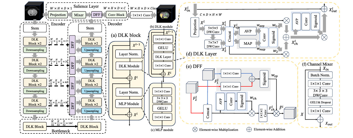
The paper, published in Biomedical Signal Processing and Control (2026), introduces three tightly integrated components: a Dynamic Large Kernel (DLK) module that captures multi-scale features via stacked large depth-wise convolutions, a Dynamic Feature Fusion (DFF) module that merges encoder and decoder features intelligently rather than naively, and a Salience layer that retrieves fine-grained, pixel-level information that hierarchical architectures would otherwise discard in their early downsampling steps. Together, the three components address complementary blind spots in every major architecture that came before — CNNs, Vision Transformers, and their hybrids alike.
The results are hard to argue with: on three fundamentally different 3D segmentation tasks — abdominal multi-organ, brain tumor, and hepatic vessel — D-Net beats every state-of-the-art model it was compared to, and it does so while using fewer parameters and less computation than most of its competitors. That combination of accuracy and efficiency is rare enough to be worth understanding carefully.
The Problem with Every Architecture Before This One
Before understanding what D-Net does, it helps to understand why every existing approach leaves something on the table.
Standard convolutional neural networks like U-Net and its variants are excellent at extracting local, spatially precise features. Their sliding-window kernels respect the neighborhood structure of images, which matters enormously when you need to trace the thin wall between a kidney and surrounding fat, or follow the winding path of a hepatic vessel. But CNNs are fundamentally limited in their ability to integrate global context. They see the local neighborhood and miss the forest.
Vision Transformers (ViTs) flip the problem. Their attention mechanism gives them a global receptive field from the start — the model can, in principle, link a pixel in the top-left corner to another in the bottom-right without any intermediate steps. But that global power comes with two costs. First, the quadratic complexity of self-attention makes applying it to high-resolution 3D volumes brutally expensive. Second, ViTs are surprisingly poor at preserving fine spatial detail. Because they first downsample input images into lower-dimensional patches, the pixel-level information needed to accurately trace organ boundaries gets smeared and lost before the model ever processes it.
Hierarchical ViTs like Swin Transformer tried to reconcile these tradeoffs by approximating self-attention locally, achieving linear complexity while retaining some global awareness. And hybrid CNN-ViT models tried to combine both approaches. But even the best hybrids tended to inherit residual weaknesses from both parents. The CNN portion struggled to model long-range dependencies. The ViT portion struggled to recover the local, boundary-level precision that clinical segmentation demands.
The researchers behind D-Net identified three specific gaps in prior work: the inability of CNNs with fixed single-scale kernels to handle organs with wildly different shapes and sizes; the loss of low-level features in ViT architectures due to early downsampling; and the crude feature fusion happening at skip connections, where encoder and decoder features were typically just concatenated without any mechanism to select which information actually mattered.
CNNs capture local detail but miss global context. Transformers capture global context but lose fine-grained spatial precision. D-Net attacks all three gaps simultaneously — multi-scale feature extraction, low-level feature recovery, and intelligent feature fusion — without inflating computational cost.
Dynamic Large Kernels: Teaching the Network to See at Multiple Scales at Once
The first core contribution is the Dynamic Large Kernel (DLK) module, and the central idea is deceptively simple: instead of using a single convolutional kernel of one fixed size, cascade two large depth-wise kernels of different sizes and dilation rates so their effective receptive fields compound.
Specifically, D-Net uses a 5×5×5 depthwise convolution with dilation 1, followed by a 7×7×7 depthwise convolution with dilation 3. The second kernel’s dilation rate effectively expands its reach, so the combined layer has an effective receptive field of approximately 23×23×23 voxels — far larger than what either kernel could achieve alone, but achieved with far fewer parameters than a naive 23×23×23 convolution would require. The cascaded design means that the features extracted by the deeper kernel are already conditioned on the output of the shallower one, creating a nested contextual hierarchy rather than a parallel collection of independent views.
But enlarging the receptive field alone is only half the story. The DLK layer also uses a dynamic selection mechanism to decide, at inference time, which of the two kernels’ contributions are most informative for the current input patch. Average pooling and max pooling along channels capture a compact global spatial summary, which is fed through a 7×7×7 convolutional layer followed by a sigmoid to generate spatially varying weights \(w_1\) and \(w_2\). These weights adaptively calibrate the contributions of the two kernel streams before combining them:
X_ch = (w₁ ⊗ X_sp) ⊕ (w₂ ⊗ X_sp)
w_ch = Sigmoid(Conv1×1×1(AvgPool(X_ch)))
X_out = w_ch ⊗ X_ch + X_in // residual connection
A channel-wise importance score \(w_{ch}\) further highlights the most informative features before the residual connection folds the result back into the main data flow. The whole operation adds only about 8% to parameter count and 2% to FLOPs compared to a single-scale 5×5×5 kernel — a remarkably cheap upgrade for a meaningful gain in representational power.
Dynamic Feature Fusion: Stop Concatenating, Start Selecting
The second major contribution tackles a problem that has been sitting quietly in U-Net-style architectures since 2015: the skip connection. The classic approach takes the encoder feature map at a given resolution and simply concatenates it with the upsampled decoder feature map from the same resolution, then feeds the doubled-channel tensor into the next convolutional block. It works, but it’s dumb — every feature is treated equally, regardless of whether it actually helps reconstruct the segmentation at that level.
The Dynamic Feature Fusion (DFF) module replaces blind concatenation with a two-stage adaptive selection process. First, it extracts global channel information \(w_{ch}\) by applying average pooling across spatial dimensions, a 1×1×1 convolution, and a sigmoid — a compact descriptor of which channels in the fused feature map carry the most signal. This information guides a convolutional layer that selectively preserves the important features while discarding noise:
F = Concat([F₁; F₂]) // F₁: encoder, F₂: upsampled decoder
w_ch = Sigmoid(Conv₁(AvgPool(F)))
F_ch = Conv₁(w_ch ⊗ F) // channel-calibrated features
// Spatial-guided recalibration
w_sp = Sigmoid(Conv₁(F₁) ⊕ Conv₁(F₂))
F̂ = w_sp ⊗ F_ch // final adaptively fused output
Then a spatial selection step identifies which spatial regions in the fused map deserve emphasis, using 1×1×1 convolutions applied separately to each input branch, summed and passed through sigmoid to generate a spatial attention map \(w_{sp}\). The output is a feature tensor that has been calibrated both across channels and across space — meaning the network actively focuses on the parts of the image that matter most for that stage of reconstruction.
When DFF was plugged into nnU-Net, Conv-ViT, and DLK-ViT as a drop-in replacement for standard concatenation, it consistently improved segmentation accuracy by 1 to 2 Dice points. Comparing it against Attentional Feature Fusion (AFF), a previous competitive fusion method, DFF pulled ahead by 2 to 4 Dice points across all three backbones — a substantial margin for a module that adds less than 0.1G FLOPs. It also has an unexpected side effect when incorporated into nnU-Net: because DFF maintains the original channel count during fusion rather than doubling it through concatenation, the downstream convolutional blocks become smaller, actually reducing total parameter count by about 10%.
“Instead of aggregating kernels in parallel as in Atrous Spatial Pyramid Pooling, we propose to sequentially aggregate multiple large kernels to enlarge receptive fields, thus capturing richer contextual information.” — Yang et al., Biomedical Signal Processing and Control 113 (2026) 108837
The Salience Layer: Rescuing the Information That Gets Lost First
The third contribution might be the most quietly important of the three, because it addresses a limitation that the community has largely accepted as an unavoidable cost of using hierarchical architectures.
All hierarchical ViTs begin by downsampling the input image through a convolutional stem — typically with a stride of 4 — before any meaningful feature extraction occurs. The logic is sound for image classification: reducing resolution early keeps computation tractable and forces the model to build abstract representations quickly. But for segmentation, which is a pixel-wise prediction task, this early discarding of information is genuinely damaging. The fine-grained boundary cues, texture gradients, and subtle intensity variations that distinguish one neighboring organ from another are encoded at full resolution. Once you’ve downsampled those away, no amount of clever upsampling in the decoder can fully recover them.
Some prior models have partially addressed this by adding convolutional blocks at the first decoder layer that process the original image, but the approach has never been clearly conceptualized or systematically studied. The Salience layer in D-Net is a deliberate, principled answer to the problem.
It operates at the full input resolution, running a parallel branch alongside the main encoder-decoder pipeline. A channel projection block first normalizes and compresses the input, then a Channel Mixer — the core of the layer — applies a global-receptive-field operation that lets features interact across all channels simultaneously. The Channel Mixer expands the channel dimension by a factor of 4 with a 1×1×1 convolution, applies a 3×3×3 depth-wise convolution with GELU activation to mix spatial information, and compresses back to the original channel count. The resulting low-level features are then fused into the decoder via a DFF module at the appropriate resolution, enriching the model’s reconstruction with fine-grained spatial cues that would otherwise be absent.
C×H×W×D
Channel proj → C/2
dilation=1 → X₁
dilation=3 → X₂
w₁,w₂ via Sigmoid
ERF ≈ 23×23×23
The ablation results were striking. Removing the Salience layer from D-Net entirely dropped performance by 2.2 Dice points. Replacing the Channel Mixer with a simple stack of two 3×3×3 convolutional layers — the approach used in prior models like DS-TransUNet — achieved slightly lower accuracy while adding 17% more FLOPs. The Channel Mixer achieves more with less, because its global receptive field lets it recognize repeating patterns across the full image volume without the local blindness that small kernels impose.
What the Numbers Actually Show
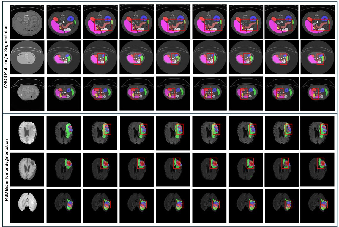
D-Net was evaluated on three benchmark tasks: abdominal multi-organ segmentation using the AMOS 2022 dataset (300 CT scans, 15 organs), brain tumor segmentation using the MSD dataset (484 multi-modal MRI scans), and hepatic vessel-tumor segmentation from the same MSD collection (303 CT scans). Five-fold cross-validation was used throughout, ensuring that results reflect genuine generalization rather than lucky splits.
AMOS Multi-Organ Segmentation
On the 15-class AMOS task, D-Net achieved a mean Dice score of 89.67 — the best result among 11 competing methods, with the lowest standard deviation (12.56), indicating consistently reliable performance rather than high variance driven by easy cases. For context, the next best method (Att U-Net) achieved 87.56, and the popular nnU-Net came in at 87.39. D-Net reached 89.67 with only 39.28M parameters and 200.13G FLOPs, compared to nnU-Net’s 68.38M parameters and 357.13G FLOPs. That’s 43% fewer parameters and 44% fewer FLOPs, at higher accuracy — a genuinely unusual combination.
The gains were especially pronounced for clinically difficult structures: the gallbladder, duodenum, and adrenal glands — organs with high inter-patient variability in shape and size — showed some of the largest improvements over prior methods. These are exactly the cases where multi-scale representation and global context awareness matter most.
| Method | Mean Dice ↑ | Mean IoU ↑ | Params (M) | FLOPs (G) |
|---|---|---|---|---|
| VNet | 84.53 | 75.78 | 45.66 | 370.52 |
| nnU-Net | 87.39 | 79.81 | 68.38 | 357.13 |
| Swin UNETR | 85.15 | 76.77 | 62.19 | 329.28 |
| UX Net | 85.52 | 77.33 | 53.01 | 632.33 |
| MedNext | 84.91 | 76.43 | 11.65 | 178.05 |
| VSmTrans | 87.08 | 79.42 | 50.39 | 358.21 |
| D-Net (Ours) | 89.67 | 81.54 | 39.28 | 200.13 |
Table 1: AMOS multi-organ segmentation results. D-Net achieves the highest Dice and IoU scores while using fewer parameters and FLOPs than most competing methods. All differences are statistically significant (p < 0.01, Wilcoxon signed-rank test).
Brain Tumor and Hepatic Vessel Segmentation
On the MSD brain tumor task, D-Net achieved a mean Dice of 74.42 ± 19.57, surpassing nnU-Net (73.83), nnFormer (73.93), and VSmTrans (74.00). The margin is smaller here, reflecting a harder task with noisier labels, but D-Net’s standard deviation is meaningfully lower than most competitors — it fails less catastrophically on the hard cases. On the hepatic vessel-tumor task, which is notoriously difficult due to the thin, branching structure of vessels, D-Net reached 67.63 mean Dice, the highest recorded, with vessel-specific performance of 65.08 and tumor performance of 70.17. MedNext, arguably the strongest prior large-kernel model, achieved 66.16 overall.
D-Net achieves state-of-the-art accuracy on all three evaluation tasks simultaneously — a rare clean sweep. More importantly, it does so while being more parameter-efficient and computationally lighter than the majority of methods it outperforms, making it realistically deployable in clinical pipelines where GPU resources are constrained.
Generalization: Does It Actually Transfer?
One of the most important but frequently overlooked evaluations in medical AI is external generalization — training on one dataset and testing on a completely different one without any fine-tuning. Clinical deployment requires models that work on scanners, protocols, and patient populations they’ve never seen before. A model that scores beautifully on its training distribution but falls apart on new data is essentially useless in practice.
The D-Net authors tested generalization by training all methods on the AMOS dataset and evaluating zero-shot on the MSD spleen dataset. D-Net achieved 94.12 ± 5.76 Dice on external evaluation — the highest of any method — compared to 97.60 on the internal AMOS spleen task, giving a generalization gap of just 3.48 points. For comparison, Swin UNETR’s gap was 5.35 points, VSmTrans’s was 6.18 points, and UX Net’s was 5.24 points. The relatively small and consistent drop suggests that D-Net is learning genuinely generalizable representations rather than overfitting to dataset-specific patterns.
The paper is also refreshingly honest about failure cases. The authors identified the specific scan instances where D-Net (and every other method) struggled most, and found that these failures were shared across architectures — suggesting that certain anatomical configurations or annotation inconsistencies pose fundamental challenges rather than architecture-specific ones. In the hepatic vessel-tumor dataset, one case (hepaticvessel_075) produced near-zero Dice scores for every single method, leading the authors to hypothesize a misalignment between the raw image and its annotation — a realistic and practically important observation about the quality of benchmark data.
What This Means for the Field
D-Net’s contribution is not a single dramatic breakthrough but rather a careful synthesis of well-motivated ideas that, together, address the segmentation problem more comprehensively than any prior approach. That kind of incremental systematization is sometimes undervalued in machine learning, where the culture rewards novelty over rigor. But in medical imaging, where the goal is reliable deployment in clinical environments, systematic coverage of failure modes matters more than flashy benchmark numbers.
The DLK module shows that you don’t need to choose between multi-scale feature extraction and computational efficiency — cascading two large kernels with a dynamic selection mechanism achieves both. The DFF module shows that the skip connection bottleneck in encoder-decoder architectures can be substantially improved without expensive redesigns. And the Salience layer shows that the community has been too quick to accept the information loss from early downsampling as unavoidable.
There are also broader lessons here for the design of 3D deep learning systems. The authors’ ablation results make clear that each of these three components contributes independently to the final performance, and their interaction is roughly additive. This is a good sign for practitioners who might want to adopt individual components into their own architectures — DFF, in particular, looks like a strong candidate for a general-purpose drop-in improvement that could benefit virtually any U-Net-style pipeline.
The generalization evaluation deserves specific mention, because the gap between internal and external performance is a more clinically meaningful metric than benchmark Dice scores alone. D-Net’s smaller generalization gap suggests that its approach to feature extraction is learning representations tied to actual anatomical structure rather than scanner-specific artifacts. That’s the kind of robustness that matters when a model trained at one hospital needs to work at another.
The frank discussion of failure cases and the hypothesis about annotation errors in the MSD hepatic vessel dataset is also worth noting. It’s a reminder that benchmark performance numbers are only as reliable as the benchmarks themselves, and that careful human analysis of failure modes remains essential even as automated metrics improve.
The Bigger Picture
Medical image segmentation is one of those problems where the gap between “good enough to publish” and “good enough to deploy” remains stubbornly wide. Models that look impressive on held-out test sets frequently show disappointing real-world performance, because the datasets they were trained on don’t capture the full variability of clinical scanners, imaging protocols, and patient populations. That gap won’t be closed by any single architectural innovation.
What D-Net offers is a set of principled design choices that address several of the most common reasons models fail in practice: inadequate multi-scale representation, poor handling of thin tubular structures, semantic confusion between neighboring organs, and poor boundary delineation. None of these are fully solved problems, but D-Net makes meaningful progress on all of them simultaneously, and it does so without requiring more computation than the methods it replaces.
The code is publicly available at github.com/sotiraslab/DLK, which means the community can build directly on this work. The DLK, DFF, and Salience layer are modular enough to be integrated into existing pipelines with relatively little engineering effort. For research groups working on organ segmentation, tumor detection, or any 3D volumetric prediction task, D-Net offers a strong baseline and a rich set of ablation results that can guide architectural decisions.
In the end, the paper’s most important contribution may be precisely its modular clarity. By cleanly separating the contributions of each component and testing them systematically, the authors have given the community something rarer and more durable than a single impressive number: a toolbox, and a clear account of why each tool works.
Access the Paper and Code
D-Net is published in Biomedical Signal Processing and Control (2026). The full implementation is available on GitHub from the Sotiras Lab at Washington University in St. Louis.
Yang, J., Qiu, P., Zhang, Y., Marcus, D. S., & Sotiras, A. (2026). D-Net: Dynamic large kernel with dynamic feature fusion for volumetric medical image segmentation. Biomedical Signal Processing and Control, 113, 108837. https://doi.org/10.1016/j.bspc.2025.108837
This article is an independent editorial analysis of peer-reviewed research. The writing style is deliberately humanized and simplified for a broader technical audience. The views expressed here reflect editorial interpretation and do not represent the views of the original authors or their institutions. Diagrams shown are illustrative representations of the concepts described, not reproductions from the original paper. Always refer to the original publication for precise technical details and authoritative results.
Explore More on AI Systems Research
From medical imaging to recommendation systems and adversarial robustness — here’s more of what we cover across the site.