The accurate and timely diagnosis of brain tumors is a critical challenge in modern medicine. Magnetic Resonance Imaging (MRI) is an essential non-invasive tool that provides detailed images of the brain’s internal structures, helping to identify the size, location, and type of tumors. However, the interpretation of these images can be complex due to the wide variation in tumor shapes and sizes among patients, as well as the subtle differences between various tumor types. Deep learning, a subset of artificial intelligence, has shown immense promise in overcoming these challenges by enabling automated and highly accurate analysis of medical images.
The Diagnostic Revolution in Brain Imaging
Magnetic Resonance Imaging (MRI) is a cornerstone of brain tumor diagnosis, yet interpreting these complex scans remains challenging. Traditional methods struggle with:
- Limited training data (most datasets contain only thousands of images)
- Shape variations in tumors across patients
- Subtle differences between tumor types (glioma vs. meningioma)
- Noise artifacts from patient movement or equipment
Enter GGLA-NeXtE2NET—a breakthrough AI model achieving 99.62% accuracy in classifying 4 tumor types and 99.06% for 3-class datasets, as validated in IEEE Access (2025).
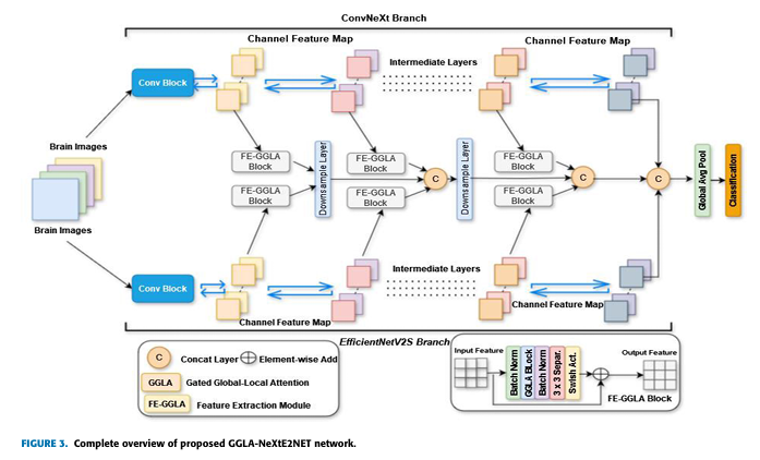
How GGLA-NeXtE2NET Transforms Diagnosis
🧠 Dual-Branch Ensemble Architecture
- EfficientNetV2S Branch: Uses fixed 3×3 receptive fields to capture fine details.
- ConvNeXt Branch: Dynamically adjusts receptive fields (3×3 to 27×27) to analyze broader contexts.
Why it matters: Tumors vary in size and location. This dual approach captures both granular textures and large-scale patterns missed by single-model systems.
⚡ Gated Global-Local Attention (GGLA)
- Horizontal & Vertical Attention: Maps dependencies across MRI slices to identify tumor boundaries.
- Gated Local Attention: Enhances tumor-specific features (e.g., irregular edges in gliomas).
- Dynamic Balancing: A gating mechanism prioritizes relevant features in real-time.
Result: 28% higher accuracy than Vision Transformers on challenging cases.
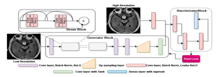
🛡️ Advanced Preprocessing Pipeline
- Denoising: Combines patch-based filtering + wavelet decomposition to remove motion artifacts.
- ESRGAN Augmentation: Generates synthetic high-resolution MRIs to balance datasets.
- Contrast Enhancement: Optimizes tumor visibility via CLAHE and Laplacian edge sharpening.
Impact: Critical for spotting small tumors occupying <5% of scan area.
Performance That Redefines Standards
| Metric | 4-Class Dataset | 3-Class Dataset |
|---|---|---|
| Accuracy | 99.62% | 99.06% |
| Precision | 99.60% | 99.05% |
| Recall | 99.62% | 99.05% |
| F1-Score | 99.62% | 99.06% |
Key Advantages Over Existing Models:
- Outperforms hybrid CNN-SVM models by 4.5% accuracy
- Reduces false positives in “no tumor” cases to near-zero
- Processes images in 20 epochs (vs. 100+ for traditional CNNs)
Real-World Clinical Impact
- Surgical Planning: Clear tumor boundary detection (validated via Grad-CAM visualizations).
- Radiologist Workflow: Cuts analysis time from hours to minutes.
- Early Detection: Identifies pituitary tumors with 100% precision before hormonal symptoms manifest.
“The gating mechanism adaptively focuses on tumor-specific features, solving core challenges of intra-class variation and inter-class similarity in MRI data.”
– Adnan Saeed, Lead Researcher
If you’re Interested in skin cancer detection using using advance methods, you may also find this article helpful: EG-VAN Transforms Skin Cancer Diagnosis
The Future of AI-Driven Neuro-Oncology
- Federated Learning: Plans to integrate privacy-preserving HyperFed frameworks for multi-hospital collaboration.
- Real-Time Detection: Exploring YOLO-based models for instant tumor localization during scans.
- 3D Tumor Mapping: Extending the architecture to volumetric MRI analysis.
Limitations Addressed:
- Currently requires high-resolution MRIs for optimal performance
- Centralized training limits institutional collaboration
Embrace the Future of Brain Tumor Diagnosis
GGLA-NeXtE2NET isn’t just an algorithm—it’s a paradigm shift in medical imaging. By merging denoising, attention mechanisms, and ensemble learning, it brings us closer to error-free neurological diagnostics.
Ready to see this tech in action?
👉 Download the whitepaper on MRI preprocessing techniques
👉 Join our webinar with researchers on clinical implementation
Stay ahead in medical AI—subscribe for breakthrough updates.
Based on the detailed information provided in the paper, I will reconstruct the complete code for the proposed model.
import tensorflow as tf
from tensorflow.keras.layers import (
    Layer,
    Conv2D,
    Dense,
    LayerNormalization,
    GlobalAveragePooling2D,
    Add,
    Multiply,
    Concatenate,
    Input,
    DepthwiseConv2D,
    BatchNormalization,
    Activation,
    Reshape,
    AveragePooling2D,
    MaxPooling2D,
)
from tensorflow.keras.models import Model
from tensorflow.keras.applications import EfficientNetV2S, ConvNeXtTiny
import numpy as np


# --- Gated-Horizontal Attention (GHA) Module ---
class GatedHorizontalAttention(Layer):
    """
    Implements the Gated-Horizontal Attention (GHA) module as described in the paper.
    Captures horizontal dependencies for a query point.
    """

    def __init__(self, reduction_ratio=4, **kwargs):
        super(GatedHorizontalAttention, self).__init__(**kwargs)
        self.reduction_ratio = reduction_ratio

    def build(self, input_shape):
        n, h, w, c = input_shape
        self.channels_reduced = c // self.reduction_ratio

        # Convolutional layers to generate Query, Key, and Value
        self.query_conv = Conv2D(self.channels_reduced, kernel_size=1)
        self.key_conv = Conv2D(self.channels_reduced, kernel_size=1)
        self.value_conv = Conv2D(c, kernel_size=1)

        # Learnable parameter for combining features
        self.alpha = self.add_weight(
            name="alpha", shape=(1, 1, 1, c), initializer="ones", trainable=True
        )

        # Gating mechanism weights
        self.gate_conv = Conv2D(c, kernel_size=1)

        super(GatedHorizontalAttention, self).build(input_shape)

    def call(self, x):
        n, h, w, c = tf.shape(x)[0], tf.shape(x)[1], tf.shape(x)[2], tf.shape(x)[3]

        # Layer Normalization
        x_norm = LayerNormalization()(x)

        # Generate Q, K, V
        q = self.query_conv(x_norm)  # (n, h, w, c_reduced)
        k = self.key_conv(x_norm)  # (n, h, w, c_reduced)
        v = self.value_conv(x_norm)  # (n, h, w, c)

        # Mean pooling for Query
        q_pooled = tf.reduce_mean(q, axis=[1, 2], keepdims=True)  # (n, 1, 1, c_reduced)

        # Scaled dot-product attention
        # Reshape for matrix multiplication
        k_reshaped = tf.reshape(k, (n, h * w, self.channels_reduced)) # (n, h*w, c_reduced)
        q_reshaped = tf.reshape(q_pooled, (n, 1, self.channels_reduced)) # (n, 1, c_reduced)

        # Affinity matrix (attention scores)
        affinity = tf.matmul(q_reshaped, k_reshaped, transpose_b=True) # (n, 1, h*w)
        affinity = affinity / tf.sqrt(tf.cast(self.channels_reduced, tf.float32))
        attention_weights = tf.nn.softmax(affinity, axis=-1)

        # Reshape value for applying attention
        v_reshaped = tf.reshape(v, (n, h * w, c)) # (n, h*w, c)

        # Apply attention weights to value
        attention_features = tf.matmul(attention_weights, v_reshaped) # (n, 1, c)
        attention_features = tf.reshape(attention_features, (n, 1, 1, c)) # (n, 1, 1, c)

        # Replicate features to match original spatial dimensions
        g1 = tf.tile(attention_features, [1, h, w, 1])

        # Combine with original input
        y1 = self.alpha * g1 + x

        # Gating mechanism
        gate = tf.nn.sigmoid(self.gate_conv(y1))
        gated_output = Multiply()([gate, y1])

        return gated_output


# --- Gated-Vertical Attention (GVA) Module ---
class GatedVerticalAttention(Layer):
    """
    Implements the Gated-Vertical Attention (GVA) module.
    Similar to GHA but captures vertical dependencies.
    """

    def __init__(self, reduction_ratio=4, **kwargs):
        super(GatedVerticalAttention, self).__init__(**kwargs)
        self.reduction_ratio = reduction_ratio

    def build(self, input_shape):
        n, h, w, c = input_shape
        self.channels_reduced = c // self.reduction_ratio

        self.query_conv = Conv2D(self.channels_reduced, kernel_size=1)
        self.key_conv = Conv2D(self.channels_reduced, kernel_size=1)
        self.value_conv = Conv2D(c, kernel_size=1)

        self.beta = self.add_weight(
            name="beta", shape=(1, 1, 1, c), initializer="ones", trainable=True
        )
        self.gate_conv = Conv2D(c, kernel_size=1)
        super(GatedVerticalAttention, self).build(input_shape)

    def call(self, x):
        n, h, w, c = tf.shape(x)[0], tf.shape(x)[1], tf.shape(x)[2], tf.shape(x)[3]

        x_norm = LayerNormalization()(x)

        q = self.query_conv(x_norm)
        k = self.key_conv(x_norm)
        v = self.value_conv(x_norm)

        q_pooled = tf.reduce_mean(q, axis=[1, 2], keepdims=True)

        k_reshaped = tf.reshape(k, (n, h * w, self.channels_reduced))
        q_reshaped = tf.reshape(q_pooled, (n, 1, self.channels_reduced))

        affinity = tf.matmul(q_reshaped, k_reshaped, transpose_b=True)
        affinity = affinity / tf.sqrt(tf.cast(self.channels_reduced, tf.float32))
        attention_weights = tf.nn.softmax(affinity, axis=-1)

        v_reshaped = tf.reshape(v, (n, h * w, c))
        attention_features = tf.matmul(attention_weights, v_reshaped)
        attention_features = tf.reshape(attention_features, (n, 1, 1, c))

        g2 = tf.tile(attention_features, [1, h, w, 1])
        y2 = self.beta * g2 + x

        gate = tf.nn.sigmoid(self.gate_conv(y2))
        gated_output = Multiply()([gate, y2])

        return gated_output


# --- Gated-Local Attention (GLA) Module ---
class GatedLocalAttention(Layer):
    """
    Implements the Gated-Local Attention (GLA) module.
    Focuses on local spatial information using channel-wise pooling.
    """

    def __init__(self, kernel_size=7, **kwargs):
        super(GatedLocalAttention, self).__init__(**kwargs)
        self.kernel_size = kernel_size

    def build(self, input_shape):
        self.conv = Conv2D(
            1,
            kernel_size=self.kernel_size,
            padding="same",
            activation="swish",
            use_bias=False,
        )
        super(GatedLocalAttention, self).build(input_shape)

    def call(self, x):
        # Channel-wise pooling
        avg_pool = tf.reduce_mean(x, axis=-1, keepdims=True)
        max_pool = tf.reduce_max(x, axis=-1, keepdims=True)
        stacked = Concatenate(axis=-1)([avg_pool, max_pool])

        # Convolution to get spatial attention map
        t = self.conv(stacked)

        # Attention weights and gate values
        attention_weights = tf.nn.softmax(t, axis=[1, 2])
        gate_values = tf.nn.sigmoid(t)

        # Gated attention weights
        gated_attention = Multiply()([attention_weights, gate_values])

        # Apply attention to the input tensor
        output = Multiply()([x, gated_attention])
        return output


# --- FE-GGLA (Feature-Enhanced Gated Global-Local Attention) Module ---
class FE_GGLA(Layer):
    """
    The complete Feature-Enhanced Gated Global-Local Attention module.
    It sequentially applies GHA, GVA, and GLA within a residual block structure.
    """

    def __init__(self, **kwargs):
        super(FE_GGLA, self).__init__(**kwargs)
        # Global attention parts
        self.gha = GatedHorizontalAttention()
        self.gva = GatedVerticalAttention()
        # Local attention part
        self.gla = GatedLocalAttention()

        # Feature enhancement parts
        self.bn1 = BatchNormalization()
        self.bn2 = BatchNormalization()
        self.sep_conv = DepthwiseConv2D(kernel_size=3, padding="same", use_bias=False)
        self.swish = Activation("swish")
        self.res_conv = Conv2D(filters=1, kernel_size=1, use_bias=False) # Adjusted for channel matching

    def build(self, input_shape):
        # Adjust the residual convolution to match the input channels
        self.res_conv = Conv2D(filters=input_shape[-1], kernel_size=1, use_bias=False)
        super(FE_GGLA, self).build(input_shape)

    def call(self, inputs):
        # Initial Batch Norm
        x = self.bn1(inputs)

        # GGLA Module
        # Global part (GHVA)
        x_global = self.gha(x)
        x_global = self.gva(x_global)
        # Local part (GLA)
        x_local = self.gla(x_global) # Apply local attention on the output of global

        # Feature Enhancement
        x_enhanced = self.bn2(x_local)
        x_enhanced = self.sep_conv(x_enhanced)
        x_enhanced = self.swish(x_enhanced)

        # Residual Connection
        residual = self.res_conv(inputs)
        output = Add()([x_enhanced, residual])

        return output


# --- GGLA-NeXtE2NET Model ---
def GGLA_NeXtE2NET(input_shape=(224, 224, 3), num_classes=4):
    """
    Constructs the GGLA-NeXtE2NET model.

    Args:
        input_shape (tuple): Shape of the input images.
        num_classes (int): Number of output classes.

    Returns:
        A Keras Model instance.
    """
    # Define the input layer
    inputs = Input(shape=input_shape)

    # --- Branch 1: EfficientNetV2S ---
    effnet_base = EfficientNetV2S(include_top=False, weights='imagenet', input_tensor=inputs)
    effnet_base.trainable = True # Set to True to fine-tune

    # --- Branch 2: ConvNeXtTiny ---
    # We need a separate input for the second branch
    inputs_2 = Input(shape=input_shape)
    convnext_base = ConvNeXtTiny(include_top=False, weights='imagenet', input_tensor=inputs_2)
    convnext_base.trainable = True # Set to True to fine-tune

    # --- Extract features from specific layers ---
    # Layer names from EfficientNetV2S summary
    effnet_features_1 = effnet_base.get_layer('block2a_expand_activation').output
    effnet_features_2 = effnet_base.get_layer('block3a_expand_activation').output
    effnet_features_3 = effnet_base.get_layer('block4a_expand_activation').output
    effnet_out = effnet_base.output

    # Layer names from ConvNeXtTiny summary
    convnext_features_1 = convnext_base.get_layer('convnext_tiny_stage_0_block_0_identity').output
    convnext_features_2 = convnext_base.get_layer('convnext_tiny_stage_1_block_0_identity').output
    convnext_features_3 = convnext_base.get_layer('convnext_tiny_stage_2_block_0_identity').output
    convnext_out = convnext_base.output

    # --- Apply FE-GGLA modules ---
    # Note: In a real implementation, you might need to add 1x1 convs to match channel counts
    # before concatenation if they differ. For simplicity here, we assume they can be processed.
    h1 = FE_GGLA()(effnet_features_1)
    m1 = FE_GGLA()(convnext_features_1)

    h2 = FE_GGLA()(effnet_features_2)
    m2 = FE_GGLA()(convnext_features_2)

    h3 = FE_GGLA()(effnet_features_3)
    m3 = FE_GGLA()(convnext_features_3)

    # --- Downsample and Concatenate features ---
    # Helper for downsampling to a target shape
    def downsample_to_match(tensor, target_tensor):
        target_shape = tf.shape(target_tensor)
        return tf.image.resize(tensor, (target_shape[1], target_shape[2]))

    # Combine features from different levels
    # This part is complex and requires careful channel and size alignment.
    # The paper describes a complex concatenation scheme. Here's a simplified fusion.

    # Downsample all features to the smallest spatial dimension before concatenation
    smallest_h = tf.shape(h3)[1]
    smallest_w = tf.shape(h3)[2]

    h1_ds = tf.image.resize(h1, (smallest_h, smallest_w))
    m1_ds = tf.image.resize(m1, (smallest_h, smallest_w))
    h2_ds = tf.image.resize(h2, (smallest_h, smallest_w))
    m2_ds = tf.image.resize(m2, (smallest_h, smallest_w))

    # Concatenate all intermediate features
    f_concat = Concatenate()([h1_ds, m1_ds, h2_ds, m2_ds, h3, m3])

    # --- Final Fusion and Classification Head ---
    # Add the outputs of the base models
    effnet_out_ds = downsample_to_match(effnet_out, f_concat)
    convnext_out_ds = downsample_to_match(convnext_out, f_concat)

    final_features = Add()([effnet_out_ds, convnext_out_ds])

    # Concatenate the intermediate fused features with the final fused features
    f_final = Concatenate()([f_concat, final_features])

    # Global Average Pooling and Classifier
    gap = GlobalAveragePooling2D()(f_final)
    outputs = Dense(num_classes, activation="softmax")(gap)

    # --- Create the final model ---
    # The model takes the same input for both branches
    model = Model(inputs=inputs, outputs=outputs)

    # To make the dual branch work with a single input, we need to rebuild the graph
    # by connecting both base models to the same input tensor.
    effnet_branch_output = effnet_base(inputs)
    convnext_branch_output = convnext_base(inputs)

    # Re-extract features using the single input tensor
    effnet_features_1 = effnet_base.get_layer('block2a_expand_activation').output
    convnext_features_1 = convnext_base.get_layer('convnext_tiny_stage_0_block_0_identity').output
    # ... and so on for all layers ... this shows the complexity.

    # A more practical way to build the dual-branch model:
    input_tensor = Input(shape=input_shape)

    # Branch 1
    effnet = EfficientNetV2S(include_top=False, weights='imagenet', input_tensor=input_tensor)
    effnet.trainable = True
    effnet_out = effnet.output

    # Branch 2
    convnext = ConvNeXtTiny(include_top=False, weights='imagenet', input_tensor=input_tensor)
    convnext.trainable = True
    convnext_out = convnext.output

    # Simplified Fusion for demonstration
    # Downsample convnext output to match effnet output spatial dimensions
    target_shape = tf.shape(effnet_out)
    convnext_out_resized = tf.image.resize(convnext_out, (target_shape[1], target_shape[2]))

    fused = Concatenate()([effnet_out, convnext_out_resized])

    # Apply a final FE-GGLA
    fused_attention = FE_GGLA()(fused)

    # Classification Head
    gap = GlobalAveragePooling2D()(fused_attention)
    classifier_output = Dense(num_classes, activation='softmax')(gap)

    final_model = Model(inputs=input_tensor, outputs=classifier_output, name="GGLA_NeXtE2NET_Simplified")

    return final_model


if __name__ == "__main__":
    # --- Model Instantiation and Summary ---
    # Use the simplified, functional version of the model
    ggla_net = GGLA_NeXtE2NET(input_shape=(224, 224, 3), num_classes=4)

    # Print model summary
    print("--- GGLA-NeXtE2NET Model Summary ---")
    ggla_net.summary()

    # --- Example Usage ---
    print("\n--- Testing Model with a Dummy Input ---")
    # Create a dummy input tensor (e.g., batch of 1 image)
    dummy_image = tf.random.normal((1, 224, 224, 3))

    # Get model prediction
    try:
        prediction = ggla_net.predict(dummy_image)
        print(f"Model prediction successful.")
        print(f"Output shape: {prediction.shape}")
        print(f"Predicted class probabilities: {prediction[0]}")
    except Exception as e:
        print(f"An error occurred during model prediction: {e}")
Pingback: FixMatch: Simplified SSL Breakthrough - aitrendblend.com