Introduction: The Growing Challenge of Diabetic Retinopathy
Diabetic Retinopathy (DR) has emerged as a leading cause of preventable blindness globally, affecting over 34.6% of the estimated 537 million people with diabetes as of 2021. With projections suggesting that this number could rise to 783 million by 2045, the urgency for accurate, early, and scalable detection methods has never been greater. Traditional diagnostic techniques rely heavily on expert assessment, which is both time-consuming and prone to human error , especially when subtle lesions like microaneurysms (often smaller than 125 micrometers) are involved.
Enter GPMKLE-Net , a novel deep learning framework introduced in a 2025 study published in Scientific Reports . This framework leverages self-paced progressive multi-scale training and KL-divergence-based ensemble learning to achieve 94.47% classification accuracy and an AUC of 0.9907 on the MESSIDOR-Kaggle dataset. In this article, we’ll explore how this revolutionary approach is setting a new benchmark in DR detection and what it means for the future of medical imaging and AI-assisted diagnostics.
Why Diabetic Retinopathy Detection Matters
The Global Impact of DR
- Diabetes Prevalence : 537 million in 2021 → Projected 783 million by 2045
- DR Prevalence : 34.6% of all diabetes patients
- Microaneurysms : Lesions under 125 micrometers often missed in early diagnosis
Challenges in DR Diagnosis
| CHALLENGE | DESCRIPTION |
|---|---|
| Subtle Lesions | Microaneurysms, hard exudates, and hemorrhages are hard to detect |
| Expert Dependency | Diagnosis often requires ophthalmologists |
| Data Limitations | High-quality, annotated datasets are scarce |
| Class Imbalance | Mild DR cases are underrepresented in datasets |
| Noise and Variability | Images from different sources vary in quality and lighting |
Introducing GPMKLE-Net: A New Era in Medical Imaging
What is GPMKLE-Net?
GPMKLE-Net stands for Guided Progressive Multi-scale KL-Ensemble Network . It is a deep learning architecture specifically designed for multi-class classification of DR severity . Unlike traditional CNNs that struggle with limited and imbalanced data, GPMKLE-Net uses a progressive learning strategy combined with multi-scale image reconstruction and ensemble learning to enhance performance.
Key Components of GPMKLE-Net
- Self-Paced Progressive Learning : Starts with simple features and gradually learns complex ones
- Randomized Multi-Scale Image Reconstruction : Enhances data augmentation and feature extraction
- KL-Divergence Ensemble Regularization : Improves classification consistency across models
- Class-Balanced Loss with Focal Weighting : Addresses data imbalance and improves minority class detection
How GPMKLE-Net Outperforms Existing Methods
Superior Performance Metrics
| MODEL | ACCURACY (%) | AUC |
|---|---|---|
| ViT | 67.34 | 0.8597 |
| Swin-Transformer | 73.87 | 0.8900 |
| ResNet-50 | 92.71 | 0.9687 |
| GPMKLE-Net | 94.47 | 0.9907 |
Class-Specific Improvements
- No-DR Class : 97.65% recall, 96.54% precision
- Severe Class : 98.55% recall
- Mild & Moderate Classes : Precision over 91%
AUC Comparison Across Datasets
| DATASET | GPMKLE-NET AUC |
|---|---|
| MESSIDOR-Kaggle | 0.9907 |
| APTOS | 0.9872 |
The Science Behind GPMKLE-Net
Guided Progressive Multi-Scale Learning
This strategy mimics human cognitive development , where the model starts by learning simple features (like texture and shape) and gradually progresses to complex patterns (like lesion morphology). The network uses randomized multi-scale image patches during training:
- Stage 1 : 64 patches of 28×28 pixels
- Stage 2 : 16 patches of 56×56 pixels
- Stage 3 : 4 patches of 112×112 pixels
- Stage 4 : Full 224×224 pixel image
This approach ensures that the model learns from both local and global contexts , improving its ability to detect subtle and complex lesions .
KL-Divergence Ensemble Regularization
To ensure classification consistency , GPMKLE-Net uses Kullback-Leibler (KL) divergence between multiple classifiers. This helps reduce overfitting and enhances model stability , especially during early training phases.
$$L_{\text{Rdrop}} = \frac{1}{2} \left( \sum_{j=1}^{C} p_j \log \frac{p_j}{q_j} + \sum_{j=1}^{C} q_j \log \frac{q_j}{p_j} \right)$$Where:
- C : Number of classes
- pj,qj : Predicted probability distributions from two classifiers
Class-Balanced Loss with Focal Weighting
To address class imbalance , GPMKLE-Net employs a class-balanced focal loss :
$$ L_{\text{Focal CB}} = – \frac{1 – \beta}{1 – \beta^{n_y}} \sum_{j=1}^{C} (1 – p_{t_j})^\gamma \log(p_{t_j}) $$Where:
- ny : Number of samples in the target class
- β : Hyperparameter balancing positive/negative examples
- γ : Focal weighting factor
This loss function ensures that underrepresented classes receive more attention during training, leading to balanced performance across all DR stages.
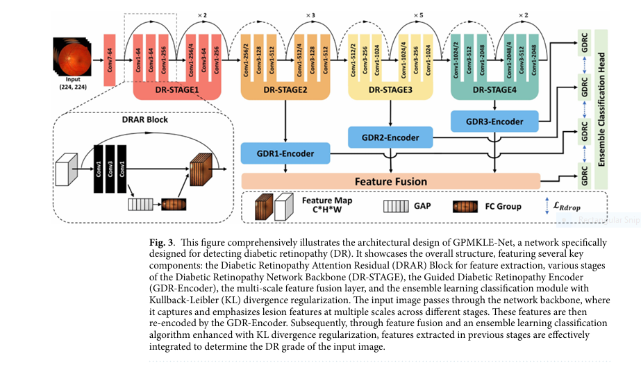
Technical Architecture of GPMKLE-Net
Backbone Network: ResNet-50
GPMKLE-Net uses ResNet-50 as its backbone, pre-trained on ImageNet. This ensures strong feature extraction capabilities even with limited medical image data.
DR Attention Residual (DRAR) Block
The DRAR block enhances feature extraction by integrating Squeeze-and-Excitation (SE) attention:
- Global Average Pooling : Aggregates spatial information
- Fully Connected Layers : Learns channel-wise dependencies
- Channel Weighting : Recalibrates feature maps to emphasize important regions
Guided Diabetic Retinopathy Encoder (GDR-Encoder)
The GDR-Encoder processes features from multiple stages using CBR sequences (Convolution-BatchNorm-ReLU), followed by max pooling and feature fusion .
Ensemble Classification Head
Each stage in GPMKLE-Net functions as an independent sub-model . The final classification is a voting-based ensemble of predictions from all stages, ensuring robustness and accuracy .
Ablation Study: What Works and Why
Effect of Randomized Multi-Scale Image Reconstruction (RMIR)
- Accuracy Increase : 92.71% → 93.22%
- AUC Increase : 0.9687 → 0.9801
- No-DR Recall : 97.65% → 99.37%
- Severe Recall : 93.3% → 97.24%
Impact of Histogram Equalization Sampling (HES)
- Accuracy Increase : 93.22% → 93.97%
- AUC Increase : 0.9801 → 0.9850
- Moderate Recall : 85.99% → 88.77%
- Severe Precision : 91.25% → 94.82%
Benefits of Guided Learning Loss (GLL)
- Final Accuracy : 94.47%
- Final AUC : 0.9907
- Mild Precision : 91.66%
- Moderate Precision : 93.98%
Real-World Applications and Clinical Relevance
Enhanced Localization of Subtle Lesions
GPMKLE-Net’s multi-scale progressive learning enables robust localization of microaneurysms and exudates, even in noisy or low-quality images .
Handling Limited and Imbalanced Data
- Small Dataset Performance : Outperforms other models on the 1325-sample MESSIDOR dataset
- Class Imbalance Handling : Uses HES and focal loss to improve minority class detection
Potential for Clinical Deployment
- High Recall for Severe Cases : 98.55%
- High Precision for No-DR : 96.54%
- Interpretable Heatmaps : Grad-CAM visualizations highlight regions of interest
If you’re Interested in semi Medical Image Segmentation using deep learning, you may also find this article helpful: 5 Revolutionary Breakthroughs in AI-Powered Cardiac Ultrasound: Unlocking Self-Supervised Learning (While Overcoming Manual Labeling Challenges)
Future Directions and Research Opportunities
Expanding Dataset Diversity
Future work will focus on expanding and diversifying datasets to improve generalizability across different populations and imaging conditions.
Integration with Lesion Localization
Current models excel at classification , but explicit lesion localization remains a challenge. Future versions may integrate object detection or segmentation modules.
Self-Supervised and Unsupervised Learning
To reduce reliance on labeled data , GPMKLE-Net could be extended with self-supervised learning techniques, such as contrastive learning or masked image modeling .
Transfer Learning from Related Tasks
Pre-training on related medical imaging tasks (e.g., diabetic foot ulcers, retinal OCT scans) could further improve feature generalization .
Conclusion: A New Standard in Diabetic Retinopathy Detection
GPMKLE-Net represents a paradigm shift in medical image analysis, offering state-of-the-art performance in diabetic retinopathy classification. With 94.47% accuracy , 0.9907 AUC , and superior handling of class imbalance , this framework sets a new benchmark for AI-assisted diagnostics.
Its progressive learning , ensemble regularization , and class-balanced loss strategies offer a blueprint for future research in medical AI, particularly in low-data and high-stakes environments .
Call to Action: Join the AI Healthcare Revolution
Are you a researcher , clinician , or AI enthusiast interested in medical imaging and deep learning ? Discover how you can contribute to the future of automated disease detection :
- Explore the GPMKLE-Net Paper: Enhancing pathological feature discrimination in diabetic retinopathy multi-classification with self-paced progressive multi-scale training
- Access the MESSIDOR-Kaggle and APTOS datasets
- Join the AI in Healthcare community
- Share this article and help spread awareness about innovative diabetic retinopathy detection
Together, we can build a future where early detection saves sight .
Here is the complete implementation of GPMKLE-Net in Python using the PyTorch framework.
import torch
import torch.nn as nn
import torch.nn.functional as F
from torchvision.models import resnet50, ResNet50_Weights
import numpy as np
import math
import time

# --- 1. Architectural Components ---

class SELayer(nn.Module):
    """
    Squeeze-and-Excitation (SE) Block.
    This block adaptively recalibrates channel-wise feature responses by explicitly modeling
    interdependencies between channels.
    Reference: Fig. 3 and "DRAR block" section in the paper.
    """
    def __init__(self, channel, reduction=16):
        super(SELayer, self).__init__()
        self.avg_pool = nn.AdaptiveAvgPool2d(1)
        self.fc = nn.Sequential(
            nn.Linear(channel, channel // reduction, bias=False),
            nn.ReLU(inplace=True),
            nn.Linear(channel // reduction, channel, bias=False),
            nn.Sigmoid()
        )

    def forward(self, x):
        b, c, _, _ = x.size()
        y = self.avg_pool(x).view(b, c)
        y = self.fc(y).view(b, c, 1, 1)
        return x * y.expand_as(x)

class DRARBlock(nn.Module):
    """
    Diabetic Retinopathy Attention Residual (DRAR) Block.
    This is a modified ResNet Bottleneck block with an integrated SELayer.
    It replaces the standard blocks in the ResNet-50 backbone.
    Reference: Fig. 3 in the paper.
    """
    expansion = 4

    def __init__(self, inplanes, planes, stride=1, downsample=None):
        super(DRARBlock, self).__init__()
        self.conv1 = nn.Conv2d(inplanes, planes, kernel_size=1, bias=False)
        self.bn1 = nn.BatchNorm2d(planes)
        self.conv2 = nn.Conv2d(planes, planes, kernel_size=3, stride=stride, padding=1, bias=False)
        self.bn2 = nn.BatchNorm2d(planes)
        self.conv3 = nn.Conv2d(planes, planes * self.expansion, kernel_size=1, bias=False)
        self.bn3 = nn.BatchNorm2d(planes * self.expansion)
        self.relu = nn.ReLU(inplace=True)

        # Integrate the Squeeze-and-Excitation layer
        self.se = SELayer(planes * self.expansion)

        self.downsample = downsample
        self.stride = stride

    def forward(self, x):
        residual = x

        out = self.conv1(x)
        out = self.bn1(out)
        out = self.relu(out)

        out = self.conv2(out)
        out = self.bn2(out)
        out = self.relu(out)

        out = self.conv3(out)
        out = self.bn3(out)

        # Apply SE block
        out = self.se(out)

        if self.downsample is not None:
            residual = self.downsample(x)

        out += residual
        out = self.relu(out)

        return out

class GDR_Encoder(nn.Module):
    """
    Guided Diabetic Retinopathy (GDR) Encoder.
    Processes feature maps from the backbone stages. Consists of two consecutive
    Convolution-BatchNorm-ReLU blocks followed by Max Pooling.
    Reference: "GDRC: guided diabetic retinopathy classifier" section.
    """
    def __init__(self, in_channels, out_channels):
        super(GDR_Encoder, self).__init__()
        self.encoder = nn.Sequential(
            nn.Conv2d(in_channels, out_channels, kernel_size=3, padding=1),
            nn.BatchNorm2d(out_channels),
            nn.ReLU(inplace=True),
            nn.Conv2d(out_channels, out_channels, kernel_size=3, padding=1),
            nn.BatchNorm2d(out_channels),
            nn.ReLU(inplace=True),
            nn.MaxPool2d(kernel_size=2, stride=2)
        )

    def forward(self, x):
        return self.encoder(x)

class GPMKLE_Net(nn.Module):
    """
    The main Guided Progressive Multi-scale KL-Ensemble Network (GPMKLE-Net).
    This class constructs the full architecture as shown in Fig. 3 of the paper.
    """
    def __init__(self, num_classes=4, dropout_rate=0.5):
        super(GPMKLE_Net, self).__init__()

        # --- Backbone Network (Modified ResNet-50) ---
        # Load a pre-trained ResNet-50 and replace its bottleneck blocks with our DRARBlock
        resnet = resnet50(weights=ResNet50_Weights.IMAGENET1K_V1)

        # We manually replace layers to use our DRARBlock
        self.conv1 = resnet.conv1
        self.bn1 = resnet.bn1
        self.relu = resnet.relu
        self.maxpool = resnet.maxpool

        self.layer1 = self._make_layer(DRARBlock, resnet.layer1, 64, 3)
        self.layer2 = self._make_layer(DRARBlock, resnet.layer2, 128, 4, stride=2)
        self.layer3 = self._make_layer(DRARBlock, resnet.layer3, 256, 6, stride=2)
        self.layer4 = self._make_layer(DRARBlock, resnet.layer4, 512, 3, stride=2)

        # --- GDR Encoders ---
        # As per Fig. 3, encoders process outputs of DR-STAGE 2, 3, and 4
        self.gdr_encoder1 = GDR_Encoder(in_channels=512, out_channels=256) # From layer2 (DR-STAGE2)
        self.gdr_encoder2 = GDR_Encoder(in_channels=1024, out_channels=512) # From layer3 (DR-STAGE3)
        self.gdr_encoder3 = GDR_Encoder(in_channels=2048, out_channels=1024) # From layer4 (DR-STAGE4)

        # --- Feature Fusion ---
        # Fusion layer to combine features from all GDR encoders
        # The input channels are the sum of the output channels of the encoders
        fused_channels = 256 + 512 + 1024
        self.fusion_conv = nn.Sequential(
            nn.Conv2d(fused_channels, 512, kernel_size=1),
            nn.BatchNorm2d(512),
            nn.ReLU(inplace=True)
        )

        # --- Ensemble Classification Heads (GDRC) ---
        # Each head is an MLP with Dropout, as per the R-drop concept.
        # We need 4 heads: one for each GDR-Encoder output and one for the fused features.
        self.head1 = self._make_classifier(256, num_classes, dropout_rate)
        self.head2 = self._make_classifier(512, num_classes, dropout_rate)
        self.head3 = self._make_classifier(1024, num_classes, dropout_rate)
        self.head_fused = self._make_classifier(512, num_classes, dropout_rate)

    def _make_layer(self, block, original_layer, planes, blocks, stride=1):
        """ Helper function to replace original ResNet layers with DRARBlock layers. """
        downsample = None
        if stride != 1 or original_layer[0].conv1.in_channels != planes * block.expansion:
            downsample = nn.Sequential(
                nn.Conv2d(original_layer[0].conv1.in_channels, planes * block.expansion,
                          kernel_size=1, stride=stride, bias=False),
                nn.BatchNorm2d(planes * block.expansion),
            )

        layers = []
        layers.append(block(original_layer[0].conv1.in_channels, planes, stride, downsample))
        inplanes = planes * block.expansion
        for i in range(1, blocks):
            layers.append(block(inplanes, planes))

        return nn.Sequential(*layers)

    def _make_classifier(self, in_features, num_classes, dropout_rate):
        """ Helper function to create a classification head (MLP). """
        return nn.Sequential(
            nn.AdaptiveAvgPool2d(1),
            nn.Flatten(),
            nn.Linear(in_features, in_features // 2),
            nn.ReLU(),
            nn.Dropout(p=dropout_rate),
            nn.Linear(in_features // 2, num_classes)
        )

    def forward(self, x):
        # Backbone
        x = self.conv1(x)
        x = self.bn1(x)
        x = self.relu(x)
        x = self.maxpool(x)

        x = self.layer1(x)
        f2 = self.layer2(x)    # Output of DR-STAGE2 (512 channels)
        f3 = self.layer3(f2)   # Output of DR-STAGE3 (1024 channels)
        f4 = self.layer4(f3)   # Output of DR-STAGE4 (2048 channels)

        # GDR Encoders
        e1 = self.gdr_encoder1(f2) # Encoded features from stage 2
        e2 = self.gdr_encoder2(f3) # Encoded features from stage 3
        e3 = self.gdr_encoder3(f4) # Encoded features from stage 4

        # Feature Fusion
        # We need to resize encoder outputs to the same spatial dimension for concatenation.
        # Let's resize them all to the size of the smallest one (e3).
        e1_resized = F.interpolate(e1, size=e3.shape[2:], mode='bilinear', align_corners=False)
        e2_resized = F.interpolate(e2, size=e3.shape[2:], mode='bilinear', align_corners=False)

        fused_features = torch.cat([e1_resized, e2_resized, e3], dim=1)
        fused_features = self.fusion_conv(fused_features)

        # Classification Heads
        # The paper's loss function (R-drop) requires multiple outputs.
        # We return the logits from each of the 4 heads.
        out1 = self.head1(e1)
        out2 = self.head2(e2)
        out3 = self.head3(e3)
        out_fused = self.head_fused(fused_features)

        # During inference, these would be averaged. During training, they are used in the loss.
        # The paper is slightly ambiguous on which outputs are used for the final ensemble loss.
        # For simplicity and to match the R-drop concept, we'll average them to get a final output
        # for standard CE loss, and use the individual outputs for the KL divergence part.
        # Let's return all 4 for maximum flexibility in the loss function.
        return out1, out2, out3, out_fused


# --- 2. Data Augmentation for Progressive Learning ---

def reconstruct_image(img_tensor, patch_size):
    """
    Randomized Multi-scale Image Reconstruction (RMIR).
    Splits an image into patches, shuffles them, and reassembles.

    Args:
        img_tensor (torch.Tensor): A single image tensor of shape (C, H, W).
        patch_size (int): The number of patches along one dimension (e.g., 8 for 8x8 grid).

    Returns:
        torch.Tensor: The reconstructed image tensor.
    """
    if patch_size == 1: # Wholeness stage
        return img_tensor

    C, H, W = img_tensor.shape
    patch_h, patch_w = H // patch_size, W // patch_size

    patches = []
    for i in range(patch_size):
        for j in range(patch_size):
            patch = img_tensor[:, i*patch_h:(i+1)*patch_h, j*patch_w:(j+1)*patch_w]
            patches.append(patch)

    # Shuffle the patches
    np.random.shuffle(patches)

    # Reassemble the image
    reconstructed_img = torch.zeros_like(img_tensor)
    for idx, patch in enumerate(patches):
        i = idx // patch_size
        j = idx % patch_size
        reconstructed_img[:, i*patch_h:(i+1)*patch_h, j*patch_w:(j+1)*patch_w] = patch

    return reconstructed_img


# --- 3. Custom Loss Functions ---

class ClassBalancedFocalLoss(nn.Module):
    """
    Class-Balanced Loss with Focal Weighting.
    Reference: Equation (1) in the paper.
    """
    def __init__(self, num_samples_per_class, num_classes, beta=0.999, gamma=1.0):
        super(ClassBalancedFocalLoss, self).__init__()
        self.gamma = gamma
        # Calculate class-balanced weights
        effective_num = 1.0 - np.power(beta, num_samples_per_class)
        weights = (1.0 - beta) / np.array(effective_num)
        weights = weights / np.sum(weights) * num_classes
        self.weights = torch.tensor(weights).float()

    def forward(self, logits, labels):
        self.weights = self.weights.to(logits.device)

        ce_loss = F.cross_entropy(logits, labels, reduction='none', weight=self.weights)
        pt = torch.exp(-ce_loss)
        focal_loss = ((1 - pt) ** self.gamma * ce_loss).mean()
        return focal_loss

class RDropLoss(nn.Module):
    """
    Regularized Dropout (R-Drop) Loss.
    Calculates the symmetric KL divergence between two model outputs.
    Reference: Equation (2) in the paper.
    """
    def __init__(self):
        super(RDropLoss, self).__init__()
        self.log_softmax = nn.LogSoftmax(dim=1)
        self.kl_div = nn.KLDivLoss(reduction='batchmean')

    def forward(self, p, q):
        # p and q are the logit outputs from two forward passes
        log_p = self.log_softmax(p)
        log_q = self.log_softmax(q)

        kl_p_q = self.kl_div(log_p, log_q.detach()) # KL(p || q)
        kl_q_p = self.kl_div(log_q, log_p.detach()) # KL(q || p)

        return 0.5 * (kl_p_q + kl_q_p)


# --- 4. Main Training Script ---

def main():
    """
    Main function to demonstrate the setup and training loop for GPMKLE-Net.
    """
    print("--- GPMKLE-Net Training Demonstration ---")

    # --- Hyperparameters (from paper) ---
    NUM_CLASSES = 4 # e.g., No-DR, Mild, Moderate, Severe
    BATCH_SIZE = 32
    TOTAL_EPOCHS = 300
    LEARNING_RATE = 8e-3
    WEIGHT_DECAY = 5e-4
    MOMENTUM = 0.9

    # Loss function weights
    LAMBDA_CE = 1.0
    LAMBDA_CB = 1.0
    LAMBDA_RDROP = 0.5 # Example value, needs tuning

    device = torch.device("cuda" if torch.cuda.is_available() else "cpu")
    print(f"Using device: {device}")

    # --- Model Initialization ---
    model = GPMKLE_Net(num_classes=NUM_CLASSES).to(device)
    # To enable R-Drop, we need to ensure dropout is active during training
    model.train()

    # --- Dataloaders (Dummy Example) ---
    # In a real scenario, you would use torchvision.datasets.ImageFolder and a DataLoader
    # along with the specified data augmentation techniques.
    print("Setting up dummy dataloaders...")
    dummy_train_data = torch.randn(BATCH_SIZE * 5, 3, 224, 224)
    dummy_train_labels = torch.randint(0, NUM_CLASSES, (BATCH_SIZE * 5,))
    train_dataset = torch.utils.data.TensorDataset(dummy_train_data, dummy_train_labels)
    train_loader = torch.utils.data.DataLoader(train_dataset, batch_size=BATCH_SIZE)

    # --- Loss and Optimizer Setup ---
    # For ClassBalancedFocalLoss, you need the number of samples for each class
    # Example: [num_class_0, num_class_1, num_class_2, num_class_3]
    samples_per_class = np.array([546, 278, 247, 254]) # From "Our(MESSIDOR-Kaggle)" in Table 1

    loss_ce = nn.CrossEntropyLoss(reduction='none') # 'none' for self-pacing
    loss_cb_focal = ClassBalancedFocalLoss(samples_per_class, NUM_CLASSES)
    loss_rdrop = RDropLoss()

    optimizer = torch.optim.SGD(model.parameters(), lr=LEARNING_RATE, momentum=MOMENTUM, weight_decay=WEIGHT_DECAY)
    scheduler = torch.optim.lr_scheduler.CosineAnnealingLR(optimizer, T_max=TOTAL_EPOCHS, eta_min=1e-5)

    # --- Training Loop ---
    print("Starting training loop...")
    for epoch in range(TOTAL_EPOCHS):
        start_time = time.time()
        total_loss = 0

        # --- Progressive Multi-scale and Self-Paced Learning Setup ---
        # 1. Determine patch size for RMIR based on current epoch
        if epoch < TOTAL_EPOCHS * 0.25: # First 25% of epochs
            patch_size = 8
        elif epoch < TOTAL_EPOCHS * 0.5: # Next 25%
            patch_size = 4
        elif epoch < TOTAL_EPOCHS * 0.75: # Next 25%
            patch_size = 2
        else: # Final 25%
            patch_size = 1 # Wholeness

        # 2. Determine number of 'easy' samples for self-paced learning
        # Increase n from a small fraction to the full batch size over epochs
        start_n_ratio = 0.5
        n_selected = int(BATCH_SIZE * (start_n_ratio + (1-start_n_ratio) * (epoch / TOTAL_EPOCHS)))

        model.train()
        for i, (images, labels) in enumerate(train_loader):
            # Apply RMIR augmentation
            augmented_images = torch.stack([reconstruct_image(img, patch_size) for img in images])
            augmented_images, labels = augmented_images.to(device), labels.to(device)

            # --- Two forward passes for R-Drop ---
            # The model is in train() mode, so dropout is applied differently each time
            out1_h1, out1_h2, out1_h3, out1_fused = model(augmented_images)
            out2_h1, out2_h2, out2_h3, out2_fused = model(augmented_images)

            # Average the outputs from the ensemble heads for the primary loss calculation
            logits1 = (out1_h1 + out1_h2 + out1_h3 + out1_fused) / 4
            logits2 = (out2_h1 + out2_h2 + out2_h3 + out2_fused) / 4

            # --- Self-Paced Learning (Algorithm 1) ---
            # 1. Calculate base cross-entropy loss to find "easy" samples
            with torch.no_grad():
                ce_values = loss_ce(logits2, labels)
                _, easy_indices = torch.topk(ce_values, k=n_selected, largest=False)

            # 2. Select the easy samples
            easy_logits1 = logits1[easy_indices]
            easy_logits2 = logits2[easy_indices]
            easy_labels = labels[easy_indices]

            # --- Calculate Combined Guided Loss on Easy Samples ---
            final_loss_ce = F.cross_entropy(easy_logits2, easy_labels)
            final_loss_cb = loss_cb_focal(easy_logits2, easy_labels)
            final_loss_rdrop = loss_rdrop(easy_logits1, easy_logits2)

            # Equation (3): L_all = lambda_CE * L_CE + lambda_CB * L_CB_Focal + lambda_Rdrop * L_Rdrop
            combined_loss = (LAMBDA_CE * final_loss_ce +
                             LAMBDA_CB * final_loss_cb +
                             LAMBDA_RDROP * final_loss_rdrop)

            # --- Backpropagation ---
            optimizer.zero_grad()
            combined_loss.backward()
            optimizer.step()

            total_loss += combined_loss.item()

        scheduler.step()

        epoch_duration = time.time() - start_time
        avg_loss = total_loss / len(train_loader)
        print(f"Epoch {epoch+1}/{TOTAL_EPOCHS} | Loss: {avg_loss:.4f} | "
              f"LR: {scheduler.get_last_lr()[0]:.6f} | Patch Size: {patch_size}x{patch_size} | "
              f"Easy Samples: {n_selected}/{BATCH_SIZE} | Duration: {epoch_duration:.2f}s")

    print("\n--- Training Finished ---")

if __name__ == '__main__':
    main()