In the high-stakes world of medical diagnostics, a single artifact in a CT scan can obscure critical details, leading to misdiagnosis or delayed treatment. For decades, radiologists have battled with image distortions caused by missing or corrupted data—problems like metal implants creating streaks or patient anatomy extending beyond the scanner’s field of view. While traditional methods offer partial solutions, they often fall short, leaving clinicians with incomplete or misleading information. Enter Latent Space Reconstruction (LSR), a groundbreaking deep learning framework that doesn’t just patch up flaws—it fundamentally rethinks how we reconstruct images from imperfect data. By leveraging the power of generative models trained on pristine scans, LSR offers a versatile, physics-aware solution that corrects artifacts at their source: the raw projection data. This article dives deep into the science behind LSR, exploring its methodology, performance against established techniques, and its transformative potential for clinical practice.
The Persistent Challenge of Artifacts in Computed Tomography
Computed tomography (CT) is a cornerstone of modern medicine, providing detailed cross-sectional views of the human body. Its core principle is elegantly simple: an X-ray source rotates around the patient, capturing projections from multiple angles. These projections, known as sinograms, are then mathematically inverted using algorithms like Filtered Backprojection (FBP) to create the final diagnostic image. However, this process relies on a fundamental assumption: that the measured data is complete and accurate. In reality, this is rarely the case.
When data is missing or corrupted, the reconstruction becomes an “ill-posed” inverse problem, meaning there isn’t enough information to guarantee a unique, artifact-free solution. Two of the most common and clinically significant sources of such problems are lateral truncation and metal artifacts.
- Lateral Truncation: Occurs when parts of the patient’s body lie outside the scanner’s Field of Measurement (FOM). This is frequent with larger patients, those not centered properly on the table, or in mobile C-arm systems with small detectors. The result is severe cupping artifacts within the FOM and a complete loss of information outside it, making diagnosis in these regions impossible.
- Metal Artifacts: Caused by metallic implants (e.g., hip replacements, dental fillings) which absorb X-rays far more than surrounding tissue. This leads to beam hardening, photon starvation, and scatter, manifesting as bright and dark streaks that can obliterate vital anatomical structures.
Traditional correction methods, while useful, have inherent limitations. Data completion techniques for truncation often rely on simplistic extrapolations that introduce new artifacts. Metal artifact reduction (MAR) methods frequently involve interpolating the corrupted sinogram region, which can lead to nonsmooth boundaries and secondary artifacts. Iterative reconstruction methods are computationally heavy and still depend on specific priors. Deep learning approaches, though powerful, are typically designed for one specific artifact type and require vast amounts of paired training data (e.g., scans with and without metal), which is difficult to obtain ethically and practically.
This is where LSR steps in, offering a paradigm shift by treating the problem as a search within a learned, structured space of possible images.
Introducing Latent Space Reconstruction (LSR): A Physics-Aware Generative Solution
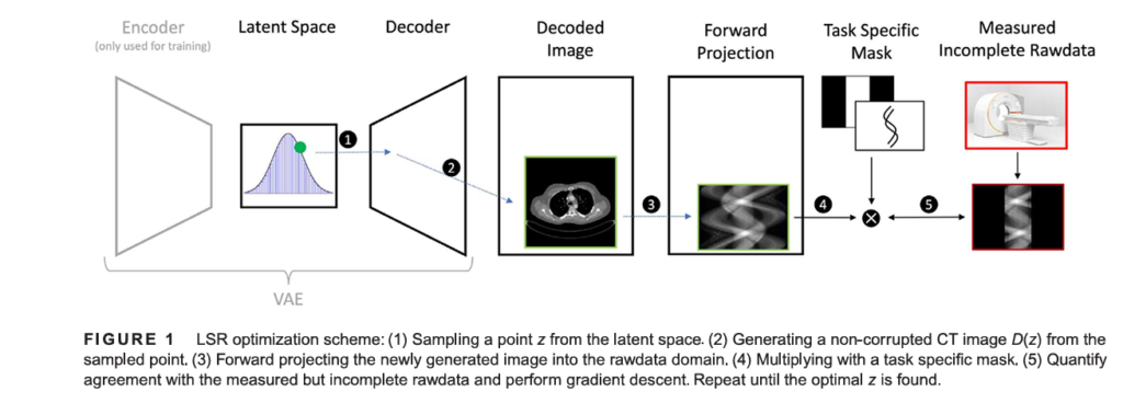
Latent Space Reconstruction (LSR) is a novel deep learning-based framework specifically designed to address the challenge of missing or corrupted data in CT imaging. Unlike many deep learning methods that operate directly on the reconstructed image or the raw sinogram, LSR works by optimizing within the latent space of a pre-trained generative model. This approach ensures that the final output is not only consistent with the measured data but also inherently realistic, as it is generated from a model that has learned the complex statistical distribution of normal, artifact-free CT images.
The core idea is elegant: instead of trying to guess what the missing data should be, LSR finds the most plausible entire image that could have produced the measured, albeit incomplete, projection data. It does this through an iterative optimization process guided by two key principles: data consistency and prior knowledge.
The Mathematical Foundation: Solving an Ill-Posed Problem
The standard CT reconstruction problem can be expressed as an inverse problem:
\[ R_f = p + n \]Where:
- f ∈ Rn is the unknown 2D or 3D CT image we want to reconstruct.
- p ∈ Rm represents the observed measurements (the sinogram).
- R (⋅): Rn → Rm is the Radon transform, modeling the forward projection process.
- n ∈ Rm is additive noise.
In cases of missing or corrupt data, some elements of p are invalid or unavailable. We denote the compromised measurement vector as q . LSR addresses this by introducing a task-specific binary mask M (α,β) ∈ {0,1}m , where M = 1 for valid measurements and M = 0 for missing/corrupted ones.
The goal of LSR is to find a latent vector z in the latent space of a generative model G (specifically, a Variational Autoencoder, or VAE, in this study) such that the forward projection of the generated image G(z) matches the measured data q as closely as possible in the regions where data exists. This is formulated as an optimization problem:
\[ z = \arg\min_{z} \, \| M(X_G(z)) – q \| \]Here, X is the forward projection operator (equivalent to R above). Once the optimal latent vector z∗ is found, the corresponding generated image G (z∗) is used to inpaint the missing regions of the sinogram. The corrected sinogram pcorrected is then:
\[ p_{\text{corrected}} = M \cdot q + (1 – M) \cdot X_G(z^{*}) \]Finally, the corrected CT image is reconstructed from pcorrected using a standard algorithm like FBP:
\[ f_{\text{corrected}} = X – \frac{1}{p_{\text{corrected}}} \]
This process explicitly retains all the original, uncorrupted measurement data (M⋅q ) and only synthesizes data for the missing regions ((1−M) ⋅ XG (z∗) ), ensuring strict data consistency—a crucial advantage over methods that blend generated components with measured data.
Why a Variational Autoencoder (VAE)?
The choice of a VAE as the generative backbone is critical to LSR’s success. A VAE consists of an encoder network that maps an input image f to a point z in a continuous, low-dimensional latent space, and a decoder network that maps z back to an image G(z) . Crucially, the VAE is trained to enforce that the latent space follows a well-behaved probability distribution (typically a multivariate Gaussian).
This regularization creates a smooth, structured latent space where:
- Close points generate similar images. Small changes in z produce small, meaningful changes in the generated image.
- Balanced sampling is possible. The model can reliably generate diverse, realistic images by sampling from the latent distribution.
This structure is essential for LSR because the optimization process needs to navigate the latent space efficiently to find the best match for the measured data. A regular autoencoder, without this regularization, would have a latent space that is often discontinuous and poorly suited for interpolation, making the optimization unstable and unreliable.
How LSR Works: A Step-by-Step Optimization Process
Implementing LSR involves a multi-stage workflow, combining machine learning with iterative numerical optimization. Here’s a detailed breakdown:
1. Training the Generative Prior
The first step is to train a VAE on a large dataset of high-quality, artifact-free CT images. In the referenced study, researchers used 94,117 axial slices from 85 adult patients scanned on a Siemens Somatom Force system at 70 kV. The VAE architecture featured residual blocks and self-attention mechanisms to handle the complexity of medical images. The model was optimized to maximize the Evidence Lower Bound (ELBO), balancing reconstruction accuracy (L1 loss) with the regularization of the latent space (KL divergence loss).
Key Takeaway: The VAE learns a comprehensive “dictionary” of normal CT anatomy. This prior knowledge is what allows LSR to generate plausible, anatomically correct images for the missing regions.
2. Defining the Task-Specific Mask
For each specific artifact correction task, a mask M is created:
- For Truncation: The mask zeros out the detector channels on the left and right edges of the sinogram, simulating a reduced FOM (e.g., 15 cm for C-arm systems).
- For Metal Artifacts: The metal is first segmented in the initial, artifact-ridden CT image using simple thresholding. Forward-projecting this segmented metal mask creates a sinogram mask Mmetal , where Mmetal=0 over the metal trace and Mmetal=1 elsewhere.
3. Iterative Latent Space Optimization
With the VAE trained and the mask defined, the core LSR algorithm begins. Starting from a randomly initialized latent vector z ∼ N (0,1) , or more efficiently, from the optimal z of the previous slice (leveraging spatial coherence), the algorithm iteratively refines z to minimize the objective function ∥M (XG (z)) − q ∥ .
This is done using gradient-based optimizers:
- Adam Optimizer: Used for the majority of iterations (around 500 steps) for fast convergence.
- L-BFGS Algorithm: Employed for the final refinement to ensure convergence to a local minimum.
Performance Insight: The study found that starting from the previous slice’s optimal z reduces the required optimization steps to about 30, significantly speeding up processing for volumetric (3D) data.
4. Sinogram Inpainting and Final Reconstruction
Once the optimal z∗ is found, the VAE generates the corresponding image G(z∗) . This image is forward-projected to create a complete sinogram XG (z∗) . The missing regions of the measured sinogram q are then replaced with the values from XG (z∗) , creating the corrected sinogram pcorrected . Finally, this corrected sinogram is reconstructed into the final diagnostic image using FBP.
Proven Performance: LSR vs. Traditional Methods
The true test of any new medical technology is its performance in real-world scenarios. The research paper provides compelling quantitative and qualitative evidence that LSR outperforms established methods for both truncation and metal artifact correction.
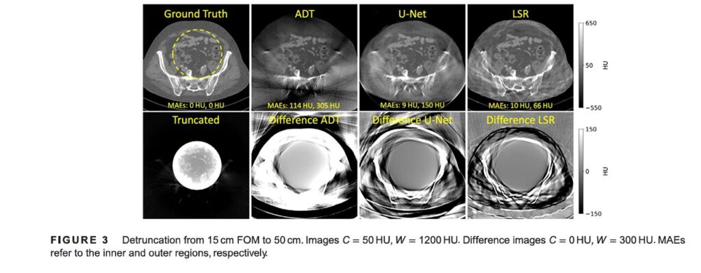
Correcting Truncation Artifacts: Extending the Field of View
In the truncation experiments, LSR was tested on simulated 15 cm FOM data, benchmarked against a classical method (Adaptive Detruncation, ADT) and a state-of-the-art deep learning method (U-Net).
- Quantitative Results (Table 1): LSR achieved the lowest Mean Absolute Error (MAE) both inside the FOM (15.0 HU) and in the sinogram domain (0.20), indicating superior data consistency. While the MAE outside the FOM was higher (102.6 HU), this is expected since this region is entirely synthesized; the value still reflects the quality of the VAE’s generation.
| METHODS | MAE INSIDE FOM [HU] | MAE OUTSIDE FOM [HU] | MAE SINOGRAM |
|---|---|---|---|
| Uncorrected | 703.5 ± 178.2 | 568.5 ± 147.9 | 1.19 ± 0.39 |
| ADT | 112.6 ± 55.5 | 313.2 ± 76.5 | 0.91 ± 0.33 |
| U-Net | 26.2 ± 24.0 | 134.4 ± 40.7 | 0.23 ± 0.17 |
| LSR | 15.0 ± 9.5 | 102.6 ± 75.5 | 0.20 ± 0.07 |
- Qualitative Results (Figure 3): Visual inspection confirmed LSR’s superiority. Images corrected by LSR showed effective suppression of cupping artifacts within the FOM and a much higher quality extension of the FOM compared to ADT and U-Net. The difference images clearly show minimal error for LSR.
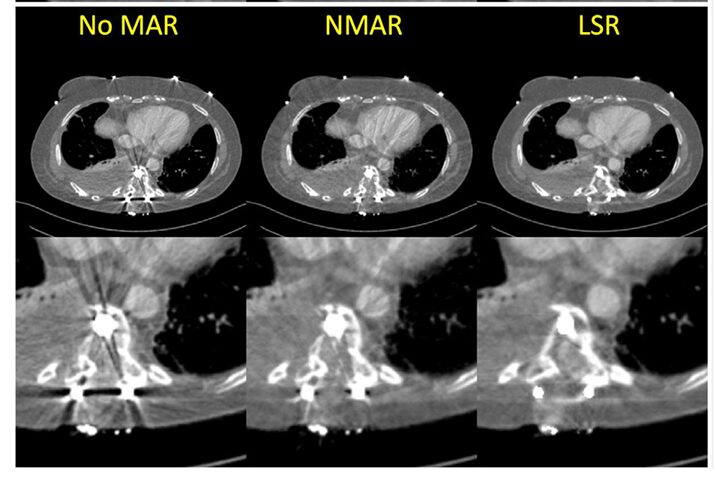
Reducing Metal Artifacts: Restoring Anatomical Detail
For metal artifacts, LSR was qualitatively compared to the widely-used Normalized Metal Artifact Reduction (NMAR) technique. Since no true artifact-free ground truth exists for patients with implants, evaluation was based on visual clarity.
- Qualitative Results (Figure 5): The results were striking. The “No MAR” image was heavily obscured by streaks. NMAR reduced the artifacts but left noticeable residual streaks near the metal. The LSR-corrected image demonstrated the most effective reduction, revealing clear, previously hidden anatomical structures and tissue details around the implant.
Important Caveat: The authors note that LSR can sometimes introduce new, tangent-oriented streak artifacts if the transition between the original and inpainted sinogram data is not perfectly smooth. This highlights an area for future improvement in the optimization or masking strategy.
Image Description: Figure 5 shows three side-by-side comparisons for two different patients with metal implants: “No MAR,” “NMAR,” and “LSR.” The LSR images clearly show reduced streaking and improved visibility of surrounding tissues.
Advantages, Limitations, and Future Directions
LSR represents a significant leap forward in CT artifact correction, but like any emerging technology, it comes with strengths and challenges.
Key Strengths of LSR
- Versatility: This is LSR’s most profound advantage. The same VAE model, trained once on clean data, can be applied to correct any type of missing or corrupted data problem—truncation, metal, limited-angle, etc.—without retraining. This generalizability is unmatched by most current methods.
- Data Consistency: By explicitly preserving the measured data and only inpainting missing regions, LSR ensures the final reconstruction is physically grounded.
- High-Quality Output: The use of a generative prior produces anatomically plausible images, leading to superior visual quality and diagnostic confidence compared to purely mathematical or interpolation-based methods.
- Generalization Potential: The study demonstrated that LSR trained on 70kV data could effectively correct artifacts in CBCT scans taken at 125kV and 140kV, suggesting robustness across different imaging protocols.
Current Limitations
- Computational Cost: The iterative optimization process is slow. On an NVIDIA GTX 3090, it takes approximately 4.3 seconds for 1000 steps. While sufficient for research, this speed is not yet suitable for time-sensitive clinical workflows. Future work must focus on accelerating the inference time.
- Dependence on Training Data: The quality of LSR’s output is directly tied to the diversity and representativeness of the VAE’s training data. The study noted that the VAE occasionally generated artifacts resembling objects from the training set (like a non-existent table), indicating a need for more diverse datasets that include variations in patient anatomy, scanner types, and noise/scatter characteristics.
Future Research Pathways
To overcome these limitations and unlock LSR’s full potential, several research directions are promising:
- Algorithmic Speedups: Exploring faster optimizers, warm-start strategies, or even replacing the iterative optimization with a learned mapping.
- Enhanced Training Data: Incorporating data from various CT systems (especially CBCT), including scans with varying levels of scatter and noise, to improve robustness.
- Advanced Modeling: Integrating explicit physical models of scatter or beam hardening into the forward projection step during optimization to further improve realism.
- Extension to 3D: Developing efficient 3D optimization strategies to handle volumetric data more coherently than slice-by-slice processing.
Conclusion: The Future of Artifact-Free CT Imaging is Here
Latent Space Reconstruction is not merely another incremental improvement in medical imaging; it is a foundational shift in how we think about solving ill-posed inverse problems. By harnessing the power of deep generative models to encode the rich prior knowledge of human anatomy, LSR provides a unified, physics-aware, and highly effective framework for correcting a wide array of CT artifacts. Its ability to extend the field of view for truncated scans and restore clarity around metal implants translates directly into better patient care, enabling more accurate diagnoses and safer, more effective treatments.
While computational speed remains a hurdle for immediate clinical deployment, the trajectory is clear. As hardware advances and algorithms become more efficient, LSR is poised to become a standard tool in the radiologist’s arsenal. The research presented here is a powerful proof of concept, demonstrating that the future of CT imaging lies not in ever-more-complex reconstruction algorithms, but in intelligent, data-driven methods that learn from the vast repository of existing medical knowledge.
Call to Action:
- Radiologists & Clinicians: Are you encountering challenging cases with truncation or metal artifacts? Share your experiences in the comments below. What specific clinical scenarios do you believe would benefit most from a technology like LSR?
- Researchers & Engineers: The path forward for LSR is collaborative. If you’re working on accelerating deep learning inference, improving generative models for medical data, or developing advanced physical models for CT, let’s connect. How can we collectively tackle the computational bottleneck?
- Patients & Advocates: Understanding the technology behind your scans empowers you. Bookmark this article and share it with your healthcare providers to spark conversations about the cutting-edge tools being developed to make your diagnostic images clearer and more reliable.
The quest for artifact-free imaging is ongoing, but with innovations like Latent Space Reconstruction, we are closer than ever to achieving it.
- Download paper Here.
Below is the complete code of LSR implementation for image reconstruction.
import torch
import torch.nn as nn
import torch.nn.functional as F
import torch.optim as optim
from torch.utils.data import Dataset, DataLoader
import numpy as np
from skimage.transform import radon, iradon
from scipy.optimize import minimize
import matplotlib.pyplot as plt


class SelfAttention(nn.Module):
    """Multi-head self-attention mechanism"""
    def __init__(self, channels, num_heads=8):
        super().__init__()
        self.channels = channels
        self.num_heads = num_heads
        self.head_dim = channels // num_heads

        assert channels % num_heads == 0, "channels must be divisible by num_heads"

        self.query = nn.Linear(channels, channels)
        self.key = nn.Linear(channels, channels)
        self.value = nn.Linear(channels, channels)
        self.fc_out = nn.Linear(channels, channels)

    def forward(self, x):
        # x shape: (batch_size, channels, height, width)
        batch_size, channels, height, width = x.shape

        # Reshape for attention: (batch_size, channels, height*width)
        x_reshaped = x.view(batch_size, channels, -1)  # (batch, channels, h*w)
        x_reshaped = x_reshaped.transpose(1, 2)  # (batch, h*w, channels)

        # Compute queries, keys, values
        queries = self.query(x_reshaped)  # (batch, h*w, channels)
        keys = self.key(x_reshaped)
        values = self.value(x_reshaped)

        # Reshape for multi-head attention
        queries = queries.view(batch_size, -1, self.num_heads, self.head_dim).transpose(1, 2)
        keys = keys.view(batch_size, -1, self.num_heads, self.head_dim).transpose(1, 2)
        values = values.view(batch_size, -1, self.num_heads, self.head_dim).transpose(1, 2)
        # shapes: (batch, num_heads, h*w, head_dim)

        # Compute attention scores
        scores = torch.matmul(queries, keys.transpose(-2, -1)) / np.sqrt(self.head_dim)
        attention_weights = F.softmax(scores, dim=-1)

        # Apply attention to values
        context = torch.matmul(attention_weights, values)  # (batch, num_heads, h*w, head_dim)

        # Concatenate heads
        context = context.transpose(1, 2).contiguous()  # (batch, h*w, num_heads, head_dim)
        context = context.view(batch_size, -1, channels)  # (batch, h*w, channels)

        # Final linear layer
        output = self.fc_out(context)  # (batch, h*w, channels)
        output = output.transpose(1, 2)  # (batch, channels, h*w)
        output = output.view(batch_size, channels, height, width)  # (batch, channels, h, w)

        # Residual connection
        return output + x


class ResidualBlock(nn.Module):
    """Residual block for VAE with self-attention"""
    def __init__(self, channels, use_attention=False):
        super().__init__()
        self.conv1 = nn.Conv2d(channels, channels, 3, padding=1)
        self.conv2 = nn.Conv2d(channels, channels, 3, padding=1)
        self.bn1 = nn.BatchNorm2d(channels)
        self.bn2 = nn.BatchNorm2d(channels)
        self.attention = SelfAttention(channels, num_heads=8) if use_attention else None

    def forward(self, x):
        residual = x
        out = F.relu(self.bn1(self.conv1(x)))
        out = self.bn2(self.conv2(out))
        out = out + residual
        out = F.relu(out)

        if self.attention is not None:
            out = self.attention(out)

        return out


class VAEEncoder(nn.Module):
    """VAE Encoder: 256x256 or 512x512 -> latent_dim with strategic self-attention"""
    def __init__(self, latent_dim=128, input_channels=3):
        super().__init__()
        self.latent_dim = latent_dim

        # Initial conv: C -> 32
        self.conv1 = nn.Conv2d(input_channels, 32, 3, stride=1, padding=1)
        self.bn1 = nn.BatchNorm2d(32)

        # Downsampling path
        self.conv2 = nn.Conv2d(32, 32, 3, stride=2, padding=1)  # H/2 x W/2
        self.res_block1 = ResidualBlock(32, use_attention=False)

        self.conv3 = nn.Conv2d(32, 64, 3, stride=2, padding=1)  # H/4 x W/4
        self.res_block2 = ResidualBlock(64, use_attention=False)

        self.conv4 = nn.Conv2d(64, 128, 3, stride=2, padding=1)  # H/8 x W/8
        self.res_block3 = ResidualBlock(128, use_attention=False)

        self.conv5 = nn.Conv2d(128, 128, 3, stride=2, padding=1)  # H/16 x W/16
        self.res_block4 = ResidualBlock(128, use_attention=False)

        # Bottleneck attention (only here - cheapest computation due to small spatial dims)
        self.attention_bottleneck = SelfAttention(128, num_heads=8)

        # For 256x256: final spatial dim is 16x16, channels=128 -> 128*16*16 = 32768
        # For 512x512: final spatial dim is 32x32, channels=128 -> 128*32*32 = 131072
        self.fc_mu = nn.Linear(128 * 16 * 16, latent_dim)
        self.fc_logvar = nn.Linear(128 * 16 * 16, latent_dim)

    def forward(self, x):
        x = F.relu(self.bn1(self.conv1(x)))
        x = F.relu(self.conv2(x))
        x = self.res_block1(x)
        x = F.relu(self.conv3(x))
        x = self.res_block2(x)
        x = F.relu(self.conv4(x))
        x = self.res_block3(x)
        x = F.relu(self.conv5(x))
        x = self.res_block4(x)

        # Apply attention only at bottleneck
        x = self.attention_bottleneck(x)

        # Use reshape instead of view to handle non-contiguous tensors from attention
        x = x.reshape(x.size(0), -1)
        mu = self.fc_mu(x)
        logvar = self.fc_logvar(x)
        return mu, logvar


class VAEDecoder(nn.Module):
    """VAE Decoder: latent_dim -> 256x256 or 512x512 with strategic self-attention"""
    def __init__(self, latent_dim=128, output_channels=3):
        super().__init__()
        self.latent_dim = latent_dim

        # Unflatten: latent_dim -> 128 x 16 x 16
        self.fc = nn.Linear(latent_dim, 128 * 16 * 16)

        # Bottleneck attention (only here for efficiency)
        self.attention_bottleneck = SelfAttention(128, num_heads=8)

        # Upsampling path
        self.conv1 = nn.ConvTranspose2d(128, 128, 4, stride=2, padding=1)  # H/8 x W/8
        self.res_block1 = ResidualBlock(128, use_attention=False)

        self.conv2 = nn.ConvTranspose2d(128, 64, 4, stride=2, padding=1)  # H/4 x W/4
        self.res_block2 = ResidualBlock(64, use_attention=False)

        self.conv3 = nn.ConvTranspose2d(64, 32, 4, stride=2, padding=1)  # H/2 x W/2
        self.res_block3 = ResidualBlock(32, use_attention=False)

        self.conv4 = nn.ConvTranspose2d(32, 32, 4, stride=2, padding=1)  # H x W
        self.res_block4 = ResidualBlock(32, use_attention=False)

        self.conv_out = nn.Conv2d(32, output_channels, 3, padding=1)

    def forward(self, z):
        x = self.fc(z)
        x = x.view(-1, 128, 16, 16)

        # Apply attention only at bottleneck
        x = self.attention_bottleneck(x)

        x = F.relu(self.conv1(x))
        x = self.res_block1(x)
        x = F.relu(self.conv2(x))
        x = self.res_block2(x)
        x = F.relu(self.conv3(x))
        x = self.res_block3(x)
        x = F.relu(self.conv4(x))
        x = self.res_block4(x)
        x = torch.sigmoid(self.conv_out(x))
        return x


class VAE(nn.Module):
    """Variational Autoencoder with Strategic Bottleneck Self-Attention"""
    def __init__(self, latent_dim=128, input_channels=3):
        super().__init__()
        self.encoder = VAEEncoder(latent_dim, input_channels)
        self.decoder = VAEDecoder(latent_dim, input_channels)
        self.latent_dim = latent_dim

    def reparameterize(self, mu, logvar):
        std = torch.exp(0.5 * logvar)
        eps = torch.randn_like(std)
        return mu + eps * std

    def forward(self, x):
        mu, logvar = self.encoder(x)
        z = self.reparameterize(mu, logvar)
        recon = self.decoder(z)
        return recon, mu, logvar, z

    def encode(self, x):
        mu, logvar = self.encoder(x)
        z = self.reparameterize(mu, logvar)
        return z

    def decode(self, z):
        return self.decoder(z)


class CTDataset(Dataset):
    """Custom Dataset for loading CT scans from .npy files"""
    def __init__(self, npy_file):
        data = np.load(npy_file)
        # Convert NumPy (N, H, W, C) to PyTorch tensor (N, C, H, W)
        self.data = torch.from_numpy(data).permute(0, 3, 1, 2).float()
        print(f"Loaded data from {npy_file}. Shape: {self.data.shape}")

    def __len__(self):
        return len(self.data)

    def __getitem__(self, idx):
        # Return single tensor (for VAE, input and target are the same)
        return self.data[idx]


class CTReconstructor:
    """CT reconstruction using Radon transform"""
    def __init__(self, image_size=512, angles=None):
        self.image_size = image_size
        if angles is None:
            self.angles = np.linspace(0, 180, 720, endpoint=False)
        else:
            self.angles = angles

    def forward_project(self, image):
        """Compute sinogram using Radon transform"""
        if isinstance(image, torch.Tensor):
            image = image.cpu().numpy()
        image = np.squeeze(image)
        sinogram = radon(image, theta=self.angles, circle=False)
        return sinogram

    def inverse_project(self, sinogram):
        """Reconstruct image using filtered backprojection"""
        image = iradon(sinogram, theta=self.angles, circle=False)
        return image

    def create_truncation_mask(self, fov_mm, max_fov_mm):
        """Create mask for truncation artifact (lateral FOV limitation)"""
        pixel_size = self.image_size / max_fov_mm
        fov_pixels = int(fov_mm * pixel_size)
        mask = np.ones((self.image_size, self.image_size))
        start = (self.image_size - fov_pixels) // 2
        end = start + fov_pixels
        mask[:, :start] = 0
        mask[:, end:] = 0
        return torch.tensor(mask, dtype=torch.float32)


class LSRMethod:
    """Latent Space Reconstruction method for CT artifact correction"""
    def __init__(self, vae, device='cuda' if torch.cuda.is_available() else 'cpu',
                 num_angles=720, image_size=512):
        self.vae = vae.to(device)
        self.device = device
        self.num_angles = num_angles
        self.image_size = image_size
        self.reconstructor = CTReconstructor(image_size,
                                            np.linspace(0, 180, num_angles, endpoint=False))

    def optimize_latent_code(self, corrupted_sinogram, mask, num_steps=500,
                            learning_rate=0.01):
        """
        Optimize latent code z to match corrupted sinogram

        Args:
            corrupted_sinogram: Incomplete/corrupted measurement data
            mask: Task-specific mask (0 for measured, 1 for missing/corrupted)
            num_steps: Number of optimization steps
            learning_rate: Learning rate for Adam optimizer

        Returns:
            Optimized latent code z
        """
        # Initialize z randomly
        z = torch.randn(1, self.vae.latent_dim,
                       device=self.device, requires_grad=True)

        corrupted_sinogram_tensor = torch.tensor(corrupted_sinogram,
                                                 dtype=torch.float32,
                                                 device=self.device)
        mask_tensor = torch.tensor(mask, dtype=torch.float32, device=self.device)

        optimizer = optim.Adam([z], lr=learning_rate)

        for step in range(num_steps):
            optimizer.zero_grad()

            # Decode z to image
            image = self.vae.decode(z)

            # Forward project to sinogram
            image_np = image.squeeze().detach().cpu().numpy()
            generated_sinogram = self.reconstructor.forward_project(image_np)
            generated_sinogram_tensor = torch.tensor(generated_sinogram,
                                                     dtype=torch.float32,
                                                     device=self.device)

            # Compute loss: only on measured regions (where mask = 1)
            diff = (generated_sinogram_tensor - corrupted_sinogram_tensor) * mask_tensor
            loss = torch.mean(diff ** 2)

            loss.backward()
            optimizer.step()

            if (step + 1) % 100 == 0:
                print(f"Step {step + 1}/{num_steps}, Loss: {loss.item():.6f}")

        return z.detach()

    def correct_image(self, corrupted_sinogram, mask, num_steps=500):
        """
        Correct corrupted CT image from incomplete sinogram

        Args:
            corrupted_sinogram: Incomplete measurement data
            mask: Task-specific mask
            num_steps: Number of optimization steps

        Returns:
            Corrected image
        """
        # Optimize latent code
        z_optimal = self.optimize_latent_code(corrupted_sinogram, mask,
                                             num_steps=num_steps)

        # Generate image from optimized z
        with torch.no_grad():
            corrected_image = self.vae.decode(z_optimal)

        # Forward project to get corrected sinogram
        image_np = corrected_image.squeeze().cpu().numpy()
        corrected_sinogram = self.reconstructor.forward_project(image_np)

        # Apply mask: keep measured data, replace corrupted with generated
        corrected_sinogram = corrupted_sinogram * (1 - mask) + \
                            corrected_sinogram * mask

        # Reconstruct final image using FBP
        final_image = self.reconstructor.inverse_project(corrected_sinogram)

        return final_image, corrected_image.squeeze().cpu().numpy()


def vae_loss(recon_x, x, mu, logvar, beta=1.0):
    """VAE loss: reconstruction + KL divergence"""
    # Reconstruction loss (L2)
    recon_loss = F.mse_loss(recon_x, x, reduction='mean')

    # KL divergence
    kl_loss = -0.5 * torch.mean(1 + logvar - mu.pow(2) - logvar.exp())

    return recon_loss + beta * kl_loss, recon_loss, kl_loss


class EarlyStopping:
    """Early stopping to prevent overfitting"""
    def __init__(self, patience=10, min_delta=0.001):
        self.patience = patience
        self.min_delta = min_delta
        self.counter = 0
        self.best_loss = None
        self.best_epoch = 0

    def __call__(self, val_loss, epoch):
        if self.best_loss is None:
            self.best_loss = val_loss
            self.best_epoch = epoch
        elif val_loss < self.best_loss - self.min_delta:
            self.best_loss = val_loss
            self.counter = 0
            self.best_epoch = epoch
        else:
            self.counter += 1

        return self.counter >= self.patience


def compute_metrics(recon_x, x):
    """Compute evaluation metrics"""
    mse = F.mse_loss(recon_x, x, reduction='mean').item()
    mae = torch.mean(torch.abs(recon_x - x)).item()

    # Peak Signal-to-Noise Ratio (PSNR)
    max_val = 1.0
    psnr = 20 * np.log10(max_val) - 10 * np.log10(mse + 1e-10)

    # Structural Similarity Index (SSIM) approximation
    ssim = 1 - F.mse_loss(
        torch.nn.functional.avg_pool2d(recon_x, 4),
        torch.nn.functional.avg_pool2d(x, 4)
    ).item()

    return {'MSE': mse, 'MAE': mae, 'PSNR': psnr, 'SSIM': ssim}


def validate_vae(vae, val_loader, device='cpu'):
    """Validate VAE on validation set"""
    vae.eval()
    total_loss = 0
    total_recon_loss = 0
    total_kl_loss = 0
    all_metrics = {'MSE': [], 'MAE': [], 'PSNR': [], 'SSIM': []}

    with torch.no_grad():
        for x in val_loader:
            x = x.to(device)
            recon_x, mu, logvar, _ = vae(x)
            loss, recon_loss, kl_loss = vae_loss(recon_x, x, mu, logvar, beta=1.0)

            total_loss += loss.item()
            total_recon_loss += recon_loss.item()
            total_kl_loss += kl_loss.item()

            metrics = compute_metrics(recon_x, x)
            for key in all_metrics:
                all_metrics[key].append(metrics[key])

    avg_metrics = {key: np.mean(vals) for key, vals in all_metrics.items()}

    return {
        'loss': total_loss / len(val_loader),
        'recon_loss': total_recon_loss / len(val_loader),
        'kl_loss': total_kl_loss / len(val_loader),
        'metrics': avg_metrics
    }


def train_vae(vae, train_loader, val_loader, num_epochs=100, lr=1e-3,
             device='cuda' if torch.cuda.is_available() else 'cpu',
             checkpoint_path='vae_best.pth'):
    """Train VAE with validation"""
    vae = vae.to(device)
    optimizer = optim.Adam(vae.parameters(), lr=lr)
    scheduler = optim.lr_scheduler.StepLR(optimizer, step_size=25, gamma=0.1)
    early_stopping = EarlyStopping(patience=15, min_delta=0.001)

    history = {
        'train_loss': [], 'train_recon': [], 'train_kl': [],
        'val_loss': [], 'val_recon': [], 'val_kl': [],
        'val_mse': [], 'val_mae': [], 'val_psnr': [], 'val_ssim': []
    }

    best_val_loss = float('inf')

    for epoch in range(num_epochs):
        # Training phase
        vae.train()
        train_loss = 0
        train_recon_loss = 0
        train_kl_loss = 0

        for batch_idx, x in enumerate(train_loader):
            x = x.to(device)
            optimizer.zero_grad()

            recon_x, mu, logvar, _ = vae(x)
            loss, recon_loss, kl_loss = vae_loss(recon_x, x, mu, logvar, beta=1.0)

            loss.backward()
            torch.nn.utils.clip_grad_norm_(vae.parameters(), max_norm=1.0)
            optimizer.step()

            train_loss += loss.item()
            train_recon_loss += recon_loss.item()
            train_kl_loss += kl_loss.item()

        avg_train_loss = train_loss / len(train_loader)
        avg_train_recon = train_recon_loss / len(train_loader)
        avg_train_kl = train_kl_loss / len(train_loader)

        # Validation phase
        val_results = validate_vae(vae, val_loader, device)

        history['train_loss'].append(avg_train_loss)
        history['train_recon'].append(avg_train_recon)
        history['train_kl'].append(avg_train_kl)
        history['val_loss'].append(val_results['loss'])
        history['val_recon'].append(val_results['recon_loss'])
        history['val_kl'].append(val_results['kl_loss'])
        history['val_mse'].append(val_results['metrics']['MSE'])
        history['val_mae'].append(val_results['metrics']['MAE'])
        history['val_psnr'].append(val_results['metrics']['PSNR'])
        history['val_ssim'].append(val_results['metrics']['SSIM'])

        scheduler.step()

        # Save best model
        if val_results['loss'] < best_val_loss:
            best_val_loss = val_results['loss']
            torch.save(vae.state_dict(), checkpoint_path)
            print(f"✓ Best model saved at epoch {epoch + 1}")

        # Print progress
        print(f"Epoch {epoch + 1}/{num_epochs}")
        print(f"  Train - Loss: {avg_train_loss:.6f}, Recon: {avg_train_recon:.6f}, KL: {avg_train_kl:.6f}")
        print(f"  Val   - Loss: {val_results['loss']:.6f}, Recon: {val_results['recon_loss']:.6f}, KL: {val_results['kl_loss']:.6f}")
        print(f"  Metrics - MSE: {val_results['metrics']['MSE']:.6f}, MAE: {val_results['metrics']['MAE']:.6f}, "
              f"PSNR: {val_results['metrics']['PSNR']:.2f}, SSIM: {val_results['metrics']['SSIM']:.4f}")

        # Early stopping
        if early_stopping(val_results['loss'], epoch):
            print(f"\nEarly stopping at epoch {epoch + 1}")
            break

    # Load best model
    vae.load_state_dict(torch.load(checkpoint_path, map_location=device))
    return vae, history


def plot_training_history(history, save_path='training_history.png'):
    """Plot training and validation curves"""
    fig, axes = plt.subplots(2, 3, figsize=(15, 8))

    # Loss
    axes[0, 0].plot(history['train_loss'], label='Train', linewidth=2)
    axes[0, 0].plot(history['val_loss'], label='Val', linewidth=2)
    axes[0, 0].set_title('Total Loss')
    axes[0, 0].set_xlabel('Epoch')
    axes[0, 0].set_ylabel('Loss')
    axes[0, 0].legend()
    axes[0, 0].grid(True)

    # Reconstruction Loss
    axes[0, 1].plot(history['train_recon'], label='Train', linewidth=2)
    axes[0, 1].plot(history['val_recon'], label='Val', linewidth=2)
    axes[0, 1].set_title('Reconstruction Loss')
    axes[0, 1].set_xlabel('Epoch')
    axes[0, 1].set_ylabel('Loss')
    axes[0, 1].legend()
    axes[0, 1].grid(True)

    # KL Loss
    axes[0, 2].plot(history['train_kl'], label='Train', linewidth=2)
    axes[0, 2].plot(history['val_kl'], label='Val', linewidth=2)
    axes[0, 2].set_title('KL Divergence Loss')
    axes[0, 2].set_xlabel('Epoch')
    axes[0, 2].set_ylabel('Loss')
    axes[0, 2].legend()
    axes[0, 2].grid(True)

    # MSE
    axes[1, 0].plot(history['val_mse'], linewidth=2, color='green')
    axes[1, 0].set_title('Validation MSE')
    axes[1, 0].set_xlabel('Epoch')
    axes[1, 0].set_ylabel('MSE')
    axes[1, 0].grid(True)

    # PSNR
    axes[1, 1].plot(history['val_psnr'], linewidth=2, color='orange')
    axes[1, 1].set_title('Validation PSNR')
    axes[1, 1].set_xlabel('Epoch')
    axes[1, 1].set_ylabel('PSNR (dB)')
    axes[1, 1].grid(True)

    # SSIM
    axes[1, 2].plot(history['val_ssim'], linewidth=2, color='red')
    axes[1, 2].set_title('Validation SSIM')
    axes[1, 2].set_xlabel('Epoch')
    axes[1, 2].set_ylabel('SSIM')
    axes[1, 2].grid(True)

    plt.tight_layout()
    plt.savefig(save_path, dpi=300)
    print(f"Training history plot saved to {save_path}")
    plt.close()


# Example usage with real data
if __name__ == "__main__":
    # Hyperparameters
    device = 'cuda' if torch.cuda.is_available() else 'cpu'
    latent_dim = 128
    batch_size = 16
    num_workers = 2
    num_epochs = 50
    learning_rate = 1e-3

    print("="*70)
    print("LSR: Latent Space Reconstruction for CT Artifact Correction")
    print("With Multi-Head Self-Attention Mechanism")
    print("="*70)

    # Define file paths to your training data
    train_path = /datapath/ct-data/train_data.npy'
    val_path = '/datapath/ct-data/validation_data.npy'
    test_path = '/datapath/ct-data/test_data(1).npy'

    # Create VAE with self-attention
    print("\n[1] Creating VAE model with Strategic Bottleneck Self-Attention...")
    # Detect input channels from data
    sample_img = train_dataset[0]
    input_channels = sample_img.shape[0]
    print(f"    Detected input channels: {input_channels}")

    vae = VAE(latent_dim=latent_dim, input_channels=input_channels)
    print(f"    Device: {device}")
    print(f"    Latent dimension: {latent_dim}")
    print(f"    Self-Attention: Enabled at Bottleneck Only (8 heads)")
    print(f"    Strategy: Attention applied at smallest feature map (16x16)")
    print(f"    Model parameters: {sum(p.numel() for p in vae.parameters()):,}")

    # Load real CT datasets from .npy files
    print("\n[2] Loading real CT datasets from .npy files...")
    print(f"    Loading train data from: {train_path}")
    train_dataset = CTDataset(train_path)

    print(f"    Loading validation data from: {val_path}")
    val_dataset = CTDataset(val_path)

    print(f"    Loading test data from: {test_path}")
    test_dataset = CTDataset(test_path)

    # Create data loaders
    print("\n[3] Creating data loaders...")
    train_loader = DataLoader(train_dataset, batch_size=batch_size,
                             shuffle=True, num_workers=num_workers, pin_memory=True)
    val_loader = DataLoader(val_dataset, batch_size=batch_size,
                           shuffle=False, num_workers=num_workers, pin_memory=True)
    test_loader = DataLoader(test_dataset, batch_size=8, shuffle=False)

    print(f"    Train batches: {len(train_loader)}")
    print(f"    Val batches: {len(val_loader)}")
    print(f"    Test batches: {len(test_loader)}")

    # Train VAE with validation
    print("\n[4] Training VAE with Self-Attention on real data...")
    print(f"    Epochs: {num_epochs}, Learning Rate: {learning_rate}")
    vae, history = train_vae(vae, train_loader, val_loader,
                            num_epochs=num_epochs, lr=learning_rate,
                            device=device, checkpoint_path='vae_best_attention.pth')

    # Evaluate on test set
    print("\n[5] Evaluating on test set...")
    test_results = validate_vae(vae, test_loader, device)
    print(f"    Test Loss: {test_results['loss']:.6f}")
    print(f"    Test Recon Loss: {test_results['recon_loss']:.6f}")
    print(f"    Test KL Loss: {test_results['kl_loss']:.6f}")
    print(f"    Test MSE: {test_results['metrics']['MSE']:.6f}")
    print(f"    Test MAE: {test_results['metrics']['MAE']:.6f}")
    print(f"    Test PSNR: {test_results['metrics']['PSNR']:.2f} dB")
    print(f"    Test SSIM: {test_results['metrics']['SSIM']:.4f}")

    # Plot training history
    print("\n[6] Plotting training history...")
    plot_training_history(history, save_path='training_history_attention.png')

    # Get image dimensions from dataset
    sample_img, _ = test_dataset[0]
    img_height = sample_img.shape[1]
    img_width = sample_img.shape[2]

    # Example: Test artifact correction on test set
    print("\n[7] Testing artifact correction on real test images...")
    lsr = LSRMethod(vae, device=device, num_angles=360, image_size=img_height)

    num_correction_tests = min(3, len(test_dataset))
    correction_metrics = []

    for test_idx in range(num_correction_tests):
        print(f"\n    Test Image {test_idx + 1}/{num_correction_tests}")

        # Get test image
        test_img, _ = test_dataset[test_idx]
        # Extract first channel if multi-channel
        if test_img.shape[0] > 1:
            original_image = test_img[0].numpy()
        else:
            original_image = test_img.squeeze().numpy()

        # Normalize to [0, 1]
        original_image = (original_image - original_image.min()) / (original_image.max() - original_image.min() + 1e-8)

        # Simulate truncation artifact
        sinogram = lsr.reconstructor.forward_project(original_image)
        mask = np.ones_like(sinogram)
        mask[:, :50] = 0
        mask[:, -50:] = 0
        corrupted_sinogram = sinogram * mask

        # Reconstruct from truncated data (baseline)
        baseline_image = lsr.reconstructor.inverse_project(corrupted_sinogram)
        baseline_image = (baseline_image - baseline_image.min()) / (baseline_image.max() - baseline_image.min() + 1e-8)

        # Correct using LSR
        corrected_image, generated_image = lsr.correct_image(
            corrupted_sinogram,
            1 - mask,
            num_steps=100
        )
        corrected_image = (corrected_image - corrected_image.min()) / (corrected_image.max() - corrected_image.min() + 1e-8)

        # Compute metrics
        original_tensor = torch.tensor(original_image, dtype=torch.float32).unsqueeze(0).unsqueeze(0).to(device)
        baseline_tensor = torch.tensor(baseline_image, dtype=torch.float32).unsqueeze(0).unsqueeze(0).to(device)
        corrected_tensor = torch.tensor(corrected_image, dtype=torch.float32).unsqueeze(0).unsqueeze(0).to(device)

        baseline_metrics = compute_metrics(baseline_tensor, original_tensor)
        corrected_metrics = compute_metrics(corrected_tensor, original_tensor)

        print(f"      Baseline - MSE: {baseline_metrics['MSE']:.6f}, PSNR: {baseline_metrics['PSNR']:.2f} dB")
        print(f"      LSR+Attn - MSE: {corrected_metrics['MSE']:.6f}, PSNR: {corrected_metrics['PSNR']:.2f} dB")
        improvement = ((baseline_metrics['MSE'] - corrected_metrics['MSE']) / baseline_metrics['MSE'] * 100)
        print(f"      Improvement: {improvement:.1f}%")

        correction_metrics.append({
            'baseline': baseline_metrics,
            'corrected': corrected_metrics
        })

    # Summary
    print("\n" + "="*70)
    print("Training and Evaluation Summary:")
    print(f"  Best Val Loss: {min(history['val_loss']):.6f} @ Epoch {np.argmin(history['val_loss']) + 1}")
    print(f"  Final Train Loss: {history['train_loss'][-1]:.6f}")
    print(f"  Final Val Loss: {history['val_loss'][-1]:.6f}")
    print(f"  Best PSNR: {max(history['val_psnr']):.2f} dB @ Epoch {np.argmax(history['val_psnr']) + 1}")
    print(f"  Final SSIM: {history['val_ssim'][-1]:.4f}")
    print(f"  Model saved to: vae_best_attention.pth")
    print(f"  Training history plot saved to: training_history_attention.png")
    print("="*70)
Related posts, You May like to read
- 7 Shocking Truths About Knowledge Distillation: The Good, The Bad, and The Breakthrough (SAKD)
- 7 Revolutionary Breakthroughs in Medical Image Translation (And 1 Fatal Flaw That Could Derail Your AI Model)
- TimeDistill: Revolutionizing Time Series Forecasting with Cross-Architecture Knowledge Distillation
- HiPerformer: A New Benchmark in Medical Image Segmentation with Modular Hierarchical Fusion
- GeoSAM2 3D Part Segmentation — Prompt-Controllable, Geometry-Aware Masks for Precision 3D Editing
- Probabilistic Smooth Attention for Deep Multiple Instance Learning in Medical Imaging
- A Knowledge Distillation-Based Approach to Enhance Transparency of Classifier Models
- Towards Trustworthy Breast Tumor Segmentation in Ultrasound Using AI Uncertainty
- Discrete Migratory Bird Optimizer with Deep Transfer Learning for Multi-Retinal Disease Detection
I don’t think the title of your article matches the content lol. Just kidding, mainly because I had some doubts after reading the article.