Introduction: The Quest for Robust AI
Deep Learning (DL) has revolutionized computer vision, enabling machines to identify objects, segment images, and drive cars with astonishing accuracy. Yet, a critical Achilles’ heel remains: these models often fail dramatically when faced with data that deviates even slightly from their training set. A self-driving car trained on sunny-day images might struggle in a snowstorm; a medical diagnostic model might be fooled by a minor artifact in an X-ray.
This vulnerability to distribution shifts—such as natural image corruptions (e.g., blur, noise), adversarial attacks, or stylistic variations (e.g., cartoons vs. photos)—poses a significant barrier to deploying AI in real-world, high-stakes environments. The core issue is a lack of generalization. While models can memorize vast training datasets, they struggle to learn underlying concepts that hold under varying conditions.
Data Augmentation (DA) has emerged as a primary defense, artificially expanding training datasets by applying transformations like rotation or color jitter to existing images. However, many traditional DA methods are limited. They often rely on simple, random alterations that do not sufficiently challenge the model or teach it true invariance.
This article explores a groundbreaking solution: LayerMix. This novel DA framework systematically enhances model robustness by integrating the structural complexity of fractals into a structured, mathematically-grounded mixing pipeline. We will dissect how LayerMix works, why it’s more effective than previous methods, and present compelling evidence from benchmarks showing significant improvements in model safety and reliability.
What is Data Augmentation and Why Does Robustness Matter?
Before diving into LayerMix, it’s essential to understand the landscape of data augmentation and the specific challenges of building robust ML systems.
The Role of Data Augmentation in Deep Learning
At its core, Data Augmentation is a form of regularization. It prevents models from overfitting to the limited examples in a training set by showing them a wider variety of data. This process helps the model learn more generalizable features.
Traditional DA techniques can be broadly categorized:
- Individual Augmentations: Apply a transformation (e.g., rotation, flipping, color adjustment) to a single image.
- Multiple Augmentations: Synthesize new samples by combining multiple images, such as in MixUp (linear interpolation of images and labels) or CutMix (replacing a patch of one image with a patch from another).
The Critical Need for Model Robustness and Safety
A model’s performance on a pristine, held-out test set (“clean accuracy”) is only part of the story. Real-world performance depends on several safety metrics:
- Corruption Robustness: How well does the model handle naturally corrupted images (e.g., fog, snow, motion blur)? Benchmarks like ImageNet-C test this.
- Adversarial Robustness: Can the model resist tiny, malicious perturbations designed to fool it? Attacks like Projected Gradient Descent (PGD) probe this weakness.
- Prediction Consistency: Does the model’s prediction stay stable when an image undergoes gradual changes (e.g., zooming in)?
- Calibration: Does the model’s predicted confidence score accurately reflect its true probability of being correct? A well-calibrated model that is 90% sure should be right 90% of the time.
Achieving a balance across these metrics is the holy grail of robust deep learning.
The Evolution of Augmentation: From MixUp to Fractals
LayerMix builds upon a lineage of increasingly sophisticated DA methods. Understanding this evolution highlights its innovative contributions.
Key Milestones in Data Augmentation
- MixUp and CutMix: These methods introduced the concept of vicinal risk minimization, blending images and labels to encourage linear behavior between classes and smoother decision boundaries.
- AutoAugment & RandAugment: These approaches automated the search for optimal sequences of transformations. RandAugment simplified this by randomly selecting transformations, increasing diversity and performance.
- AugMix: This method combined the IID (Independent and Identically Distributed) augmentation stages of RandAugment with the blending concept of MixUp. It also added a Jensen-Shannon Divergence (JSD) consistency loss to ensure that the representations of augmented images did not stray too far from the original, balancing diversity with affinity to the original data manifold.
The Fractal Revolution: PixMix and IPMix
A significant leap came with the introduction of fractals. Fractals are infinitely complex, repeating patterns that are naturally rich in structure and detail.
- PixMix pioneered the use of fractals in DA. By blending training images with fractal patterns, it could generate highly diverse samples that were unlikely to conflict with the original image’s label. This provided a massive boost to diversity without causing “manifold intrusion,” where synthetic samples confuse the model. PixMix also introduced a mixture of blending methods, like arithmetic and geometric means.
- IPMix further advanced this by incorporating pixel-level and element-level mixing, creating even more diverse samples and pushing state-of-the-art robustness benchmarks.
However, these methods operated in a vast search space and often relied on additional training tricks for optimal performance. LayerMix was designed to address these limitations with a more structured and efficient pipeline.
Introducing LayerMix: A Structured Approach to Augmentation
LayerMix is an innovative DA framework designed to optimally balance affinity (preserving semantic meaning) and diversity (expanding beyond the original data manifold). It achieves this through four key innovations.
1. Pipeline Covariance: Breaking the IID Assumption
Previous pipelines like RandAugment treated each augmentation stage as independent. At each step, a transformation (e.g., rotation, color jitter) was chosen randomly. LayerMix introduces covariance between these stages.
- How it works: Instead of choosing a new random transformation for each stage, LayerMix selects one transformation type (e.g., rotation) and applies it consistently across multiple stages, varying only its magnitude.
- Mathematical Insight: This creates a dependency between stages. The joint distribution of the pipeline’s output is no longer a simple product of independent stages but rather the expected value over the chosen transformation type.
Compared to the IID approach:
This covariance structure reduces unnecessary randomness that doesn’t contribute to performance, allowing the reallocation of “diversity budget” to more effective areas, like increasing the magnitude of the transformations.
2. Fractal Augmentation: Embracing Grayscale Complexity
LayerMix uses the same dataset of 14,230 fractals as PixMix but with a critical modification: it converts them to grayscale.
- Why Grayscale? Research has shown that the structural complexity of fractals—their shapes and contours—is what provides the most benefit for pre-training and augmentation. Color information does not add significant value and can even introduce noise.
- Enhanced by Augmentation: LayerMix further augments these grayscale fractals with random horizontal and vertical flips, increasing their diversity before they are blended with training images. This simple change was found to improve robustness metrics.
3. Reweighted Blending: Strategically Balancing Methods
LayerMix uses a mixture of blending methods, but it strategically reweights their probabilities based on an ablation study of their strengths:
| Blending Method | Expression | Probability in LayerMix |
|---|---|---|
| Arithmetic Mean | Y = aZ0 + bZ1 | 33.3% |
| Geometric Mean | Y = 2a+b−1 ⋅ Z0 ⋅ Z1 | 33.3% |
| Pixel Mixing | Y = M ⊙ Z0 + (1−M) ⊙ Z1 | 16.6% |
| Element Mixing | Y = M ⊙ Z0 + (1−M) ⊙ Z1 | 16.6% |
- Finding: Arithmetic and geometric means were most effective for improving clean accuracy. Pixel-wise mixing excelled at enhancing corruption robustness.
- Strategy: By doubling the probability of the mean-based methods, LayerMix biases the pipeline towards clean accuracy while still retaining the robustness benefits of pixel-level mixing.
4. A Novel Three-Layer Pipeline Architecture
The entire LayerMix process is structured into a three-layer pipeline, as illustrated below.
Image Description (Fig. 2): A flowchart illustrating the 3-layer LayerMix pipeline. An input image is processed through correlated augmentation stages (Aug) and blending stages (Blend) with an augmented fractal. The final output is selected uniformly at random from one of three resulting samples, each with an increasing level of diversity.
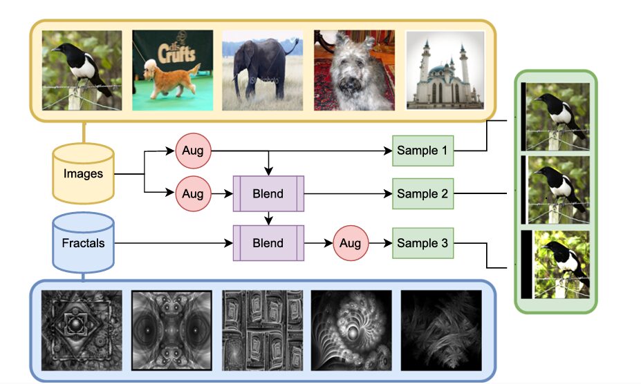
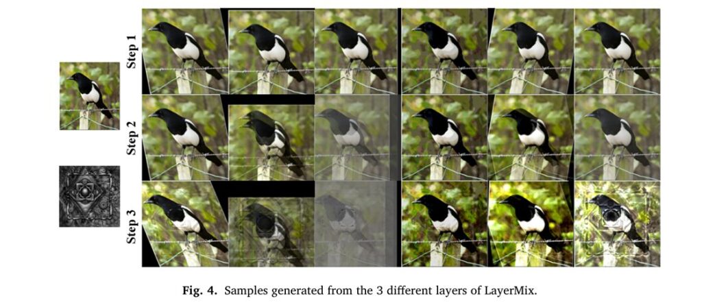
The key insight is that the three output samples possess different levels of diversity:
- Sample 1: Least diverse (closest to the original image manifold).
- Sample 2: Moderately diverse.
- Sample 3: Most diverse (due to blending with an augmented fractal).
The final augmented image is chosen uniformly at random from these three samples. This clever design provides fine-grained control over the diversity of the training data, reducing the average deviation from the original data manifold while still generating highly challenging samples when needed.
Experimental Results: How LayerMix Performs on Benchmark Tests
The true test of any DA method is its performance on standardized benchmarks. LayerMix was evaluated across multiple datasets and safety metrics against state-of-the-art competitors like AugMix, PixMix, and IPMix.
Dominant Performance on CIFAR-10 and CIFAR-100
On the CIFAR-100 dataset using a WideResNet-40-4 model, LayerMix demonstrated superior performance:
- Corruption Robustness (mCE): 30.34 (LayerMix) vs. 30.84 (IPMix) and 35.54 (PixMix). A lower mCE is better.
- Prediction Consistency (mFP): 5.55 (LayerMix) vs. 5.85 (IPMix) and 6.16 (PixMix). A lower flip probability indicates more stable predictions.
- Calibration (RMS Error): 5.92 (LayerMix) vs. 10.31 (IPMix) and 7.00 (PixMix). A lower error means the model’s confidence is better aligned with its accuracy.
These results show that LayerMix provides a more balanced improvement across all safety metrics compared to previous methods.
Table: Key Results on CIFAR-100 (WRN-40-4)
| Method | Clean Error ↓ | Corruption mCE ↓ | Adversarial Error ↓ | Consistency mFP ↓ | Calibration RMS ↓ |
|---|---|---|---|---|---|
| Baseline | 21.3 | 50.0 | 96.8 | 10.7 | 14.6 |
| AugMix | 20.6 | 35.4 | 95.6 | 6.5 | 12.5 |
| PixMix | 20.4 | 35.5 | 92.4 | 6.3 | 7.0 |
| IPMix | 20.4 | 30.8 | 95.0 | 6.0 | 10.3 |
| LayerMix | 20.7 | 30.3 | 95.5 | 5.6 | 5.9 |
Scalability and Success on ImageNet
A crucial test for any method is scalability to large, complex datasets like ImageNet. On ImageNet-200 (a 200-class subset), LayerMix continued to excel:
- Corruption Robustness: LayerMix achieved an mCE of 29.77, a 14.26% improvement over the baseline and a 3.54% improvement over the next best method (PixMix).
- Rendition Robustness (ImageNet-R): It achieved the lowest error rate (57.27), showing better performance on artistic renditions like paintings and cartoons.
- Calibration: LayerMix also produced the best-calibrated predictions on corrupted data (RMS of 4.72).
These results confirm that LayerMix’s advantages are not limited to smaller datasets but scale effectively to real-world complexity.
Conclusion and Future Directions: Building More Trustworthy AI
LayerMix represents a significant step forward in the pursuit of robust and reliable deep learning. By moving beyond random transformations to a structured, mathematically-informed augmentation pipeline, it demonstrates that how you augment data is just as important as how much you augment it.
Key Takeaways:
- Structured Beats Random: Introducing covariance between augmentation stages and strategically reweighting blending methods leads to more efficient learning.
- Complexity over Color: The structural complexity of grayscale fractals is a powerful tool for enhancing model robustness without introducing distracting color noise.
- Balanced Performance: LayerMix provides a balanced improvement across critical safety metrics—corruption robustness, adversarial robustness, prediction consistency, and calibration—making it ideal for real-world applications.
The Path Ahead
The success of LayerMix opens up several exciting avenues for future research:
- Theoretical Understanding: A deeper statistical formulation of why and how fractals work could lead to even more effective pipeline designs.
- Beyond Classification: Adapting LayerMix for object detection, segmentation, and other downstream tasks is a crucial next step.
- Extended Covariance: Applying the covariance concept to blending stages, not just augmentation stages, could yield further gains.
In a world increasingly dependent on AI, developing models that we can trust under all conditions is paramount. LayerMix provides a powerful and scalable framework for building these trustworthy systems.
Call to Action
What are your biggest challenges with model robustness? Have you experimented with data augmentation techniques like MixUp or AugMix in your projects? Share your experiences and thoughts on the future of robust AI in the comments below. For researchers and practitioners, the complete code for LayerMix is available on GitHub and paper to facilitate further experimentation and application.
Here is the end-to-end code. It includes the core LayerMix pipeline, all the necessary helper functions for augmentation and blending, a synthetic fractal generator (as the paper’s dataset is external), and a runnable example to demonstrate its usage.
import torch
import torchvision.transforms as transforms
import torchvision.transforms.v2 as T
import random
import numpy as np
from PIL import Image

# This script requires the following libraries:
# pip install torch torchvision numpy Pillow matplotlib

# --- 1. Augmentation Operations (from Paper's Table 2) ---
# A helper function that returns a list of augmentation functions parameterized by a single magnitude.
# We implement a representative subset of the transformations from Table 2.
def get_augmentations(magnitude):
    """
    Returns a list of torchvision.transforms.v2 augmentation functions.
    The strength of each transform is scaled by the magnitude parameter.

    Args:
        magnitude (int): An integer from 1-10 to control the strength of augmentations.

    Returns:
        list: A list of callable transform objects.
    """
    # Scale magnitude (1-10) to the specific ranges used in the paper.
    mag_fraction = magnitude / 10.0

    # Define ranges based on the paper's descriptions
    shear_val = mag_fraction * 0.3
    translate_val = mag_fraction * 0.33
    rotate_val = mag_fraction * 30
    # For ColorJitter, brightness range is [1-val, 1+val]. Paper's range is 0.1 to 1.9.
    brightness_val = mag_fraction * 0.9
    # Posterize bits range from 4 down to 0.
    posterize_bits = 4 - int(mag_fraction * 4)
    # Solarize threshold ranges from 1.0 down to 0.0.
    solarize_threshold = 1.0 - mag_fraction

    # Using transforms.v2 as they operate on tensors, which is required by the pipeline.
    augmentations = [
        T.RandomRotation(degrees=(-rotate_val, rotate_val)),
        T.RandomAffine(degrees=0, shear=(-shear_val, shear_val)),
        T.RandomAffine(degrees=0, translate=(translate_val, 0)),
        T.RandomAffine(degrees=0, translate=(0, translate_val)),
        T.ColorJitter(brightness=brightness_val),
        T.RandomPosterize(bits=max(1, posterize_bits)), # bits must be at least 1 for this transform
        T.RandomSolarize(threshold=solarize_threshold),
        T.RandomAutocontrast(),
        T.RandomEqualize(),
        T.Grayscale(num_output_channels=3) # Keep 3 channels for tensor compatibility
    ]
    return augmentations

# --- 2. Blending Methods (from Paper's Table 1) ---

def arithmetic_mean(img1, img2, beta):
    """Blends two images using a weighted arithmetic mean."""
    w = np.random.beta(beta, beta)
    return w * img1 + (1 - w) * img2

def geometric_mean(img1, img2, beta):
    """Blends two images using a weighted geometric mean."""
    # Add a small epsilon to avoid issues with log(0) or pow(0, neg).
    img1 = torch.clamp(img1, 1e-6)
    img2 = torch.clamp(img2, 1e-6)
    w = np.random.beta(beta, beta)
    return img1**w * img2**(1 - w)

def pixel_mixing(img1, img2, beta):
    """Blends two images using a mask at the pixel level."""
    w = np.random.beta(beta, beta)
    # Create a 2D mask and expand it to all channels
    mask_shape = (img1.shape[0], 1, img1.shape[2], img1.shape[3])
    mask = torch.bernoulli(torch.full(mask_shape, w)).to(img1.device)
    return mask * img1 + (1 - mask) * img2

def element_mixing(img1, img2, beta):
    """Blends two images using a mask at the element (pixel-channel) level."""
    w = np.random.beta(beta, beta)
    mask = torch.bernoulli(torch.full_like(img1, w)).to(img1.device)
    return mask * img1 + (1 - mask) * img2


# --- 3. Fractal Generation ---
# As the paper uses an external dataset of fractals, we generate a synthetic
# plasma fractal on-the-fly to make this script self-contained.
def generate_plasma_fractal(size, roughness=0.6):
    """
    Generates a grayscale plasma fractal image as a PyTorch tensor.

    Args:
        size (tuple): The (width, height) of the desired fractal.
        roughness (float): Controls the roughness of the fractal texture.

    Returns:
        torch.Tensor: A 3-channel grayscale fractal tensor of shape (3, H, W).
    """
    width, height = size
    points = torch.zeros((height, width), dtype=torch.float32)

    # Initialize corners
    points[0, 0] = random.random()
    points[width - 1, 0] = random.random()
    points[0, height - 1] = random.random()
    points[width - 1, height - 1] = random.random()

    step = width - 1
    while step > 1:
        half = step // 2
        # Square step
        for i in range(0, width - 1, step):
            for j in range(0, height - 1, step):
                avg = (points[j, i] + points[j + step, i] + points[j, i + step] + points[j + step, i + step]) / 4.0
                points[j + half, i + half] = avg + (random.random() - 0.5) * step / width * roughness
        # Diamond step
        for i in range(0, width - 1, half):
            for j in range((i + half) % step, height - 1, step):
                count = 0
                total = 0.0
                if i >= half: total += points[j, i - half]; count += 1
                if i < width - half: total += points[j, i + half]; count += 1
                if j >= half: total += points[j - half, i]; count += 1
                if j < height - half: total += points[j + half, i]; count += 1
                avg = total / count
                points[j, i] = avg + (random.random() - 0.5) * step / width * roughness
        step //= 2

    # Normalize to [0, 1] range
    min_val, max_val = points.min(), points.max()
    if max_val > min_val:
        points = (points - min_val) / (max_val - min_val)

    # Convert to a 3-channel tensor
    return points.unsqueeze(0).repeat(3, 1, 1)


# --- 4. The LayerMix Transform Class ---
class LayerMix(object):
    """
    LayerMix data augmentation implementation based on the research paper.
    This transform should be applied to a tensor image.
    """
    def __init__(self, magnitude=8, blending_ratio=3):
        """
        Args:
            magnitude (int): The magnitude of the augmentation operations (1-10).
            blending_ratio (float): The beta parameter for the blending distributions.
        """
        self.magnitude = magnitude
        self.blending_ratio = blending_ratio
        self.augmentations = get_augmentations(self.magnitude)

        # Reweighted blending methods (from Paper's Section 3.3 and Table 1)
        self.blending_methods = [
            (arithmetic_mean, 0.333),
            (geometric_mean, 0.333),
            (pixel_mixing, 0.166),
            (element_mixing, 0.166)
        ]
        self.blending_fns = [f[0] for f in self.blending_methods]
        self.blending_probs = [f[1] for f in self.blending_methods]

    def __call__(self, img_tensor):
        """
        Applies the LayerMix augmentation to an input tensor.

        Args:
            img_tensor (torch.Tensor): Input image tensor of shape (C, H, W).

        Returns:
            torch.Tensor: The augmented image tensor.
        """
        # The transform expects a batch, so we unsqueeze if it's a single image.
        is_batched = len(img_tensor.shape) == 4
        if not is_batched:
            img_tensor = img_tensor.unsqueeze(0)

        # --- Pipeline implementation (from Paper's Section 3.4 and Code Block 1) ---

        # 1. Randomly select the output layer (Sample 1, 2, or 3)
        step = random.randint(0, 2)

        # 2. Select a single augmentation for all stages (Pipeline Covariance, Sec 3.1)
        aug_fn = random.choice(self.augmentations)

        # --- Step 0 (produces Sample 1) ---
        img_aug = aug_fn(img_tensor)
        if step == 0:
            return img_aug.squeeze(0) if not is_batched else img_aug

        # --- Step 1 (builds towards Sample 2) ---
        img_copy = img_tensor.clone()
        img2_aug = aug_fn(img_copy)

        blending_fn_1 = random.choices(self.blending_fns, self.blending_probs, k=1)[0]

        img_blended_1 = torch.clip(
            blending_fn_1(img_aug, img2_aug, self.blending_ratio), 0, 1
        )

        if step == 1:
            return img_blended_1.squeeze(0) if not is_batched else img_blended_1

        # --- Step 2 (produces Sample 3) ---

        # 3. Prepare fractal mixing image (Fractal Augmentation, Sec 3.2)
        _, _, h, w = img_tensor.shape
        fractal_img = generate_plasma_fractal(size=(w, h)).unsqueeze(0).to(img_tensor.device)

        # Apply random flips to the fractal
        if random.random() > 0.5:
            fractal_img = T.RandomHorizontalFlip(p=1.0)(fractal_img)
        if random.random() > 0.5:
            fractal_img = T.RandomVerticalFlip(p=1.0)(fractal_img)

        blending_fn_2 = random.choices(self.blending_fns, self.blending_probs, k=1)[0]

        img_blended_2 = torch.clip(
            blending_fn_2(img_blended_1, fractal_img, self.blending_ratio), 0, 1
        )

        # Final augmentation step for Sample 3
        final_img = aug_fn(img_blended_2)

        return final_img.squeeze(0) if not is_batched else final_img


# --- 5. Example Usage ---
if __name__ == '__main__':
    print("Running LayerMix demonstration...")

    # Load a sample image from a URL
    try:
        from urllib.request import urlopen
        # Using an image from the original authors' GitHub for consistency
        url = 'https://raw.githubusercontent.com/ahmadmughees/layermix/main/assets/ILSVRC2012_val_00000023.JPEG'
        image = Image.open(urlopen(url)).convert('RGB').resize((224, 224))
        print("Sample image loaded successfully from URL.")
    except Exception as e:
        print(f"Failed to load image from URL: {e}. Creating a dummy image instead.")
        image = Image.new('RGB', (224, 224), color = (128, 64, 200))

    # Define the full transformation pipeline
    transform_pipeline = transforms.Compose([
        transforms.ToTensor(),    # 1. Convert PIL image to tensor in range [0, 1]
        LayerMix(magnitude=8, blending_ratio=3) # 2. Apply LayerMix on the tensor
    ])

    # Generate one augmented image and save it
    augmented_image_tensor = transform_pipeline(image)
    augmented_image_pil = transforms.ToPILImage()(augmented_image_tensor)

    image.save("original_image.png")
    augmented_image_pil.save("layermix_augmented_image.png")

    print("\nDemonstration complete.")
    print("Saved 'original_image.png' and a single 'layermix_augmented_image.png'.")

    # Generate and save a grid of multiple examples to showcase diversity
    try:
        import matplotlib.pyplot as plt

        fig, axes = plt.subplots(3, 4, figsize=(16, 12))
        fig.suptitle("LayerMix Augmentation Examples", fontsize=20)

        axes[0, 0].imshow(image)
        axes[0, 0].set_title("Original Image")
        axes[0, 0].axis('off')

        for i in range(3):
            for j in range(4):
                if i == 0 and j == 0: continue
                aug_img = transform_pipeline(image)
                axes[i, j].imshow(transforms.ToPILImage()(aug_img))
                axes[i, j].set_title(f"Example {i*4+j}")
                axes[i, j].axis('off')

        plt.tight_layout(rect=[0, 0, 1, 0.96])
        plt.savefig("layermix_grid.png")
        print("Saved 'layermix_grid.png' with a grid of augmented examples.")
    except ImportError:
        print("\nMatplotlib not found. Skipping grid generation.")
        print("To generate the grid, please install it: pip install matplotlib")
Related posts, You May like to read
- 7 Shocking Truths About Knowledge Distillation: The Good, The Bad, and The Breakthrough (SAKD)
- 7 Revolutionary Breakthroughs in Medical Image Translation (And 1 Fatal Flaw That Could Derail Your AI Model)
- DeepSPV: Revolutionizing 3D Spleen Volume Estimation from 2D Ultrasound with AI
- ACAM-KD: Adaptive and Cooperative Attention Masking for Knowledge Distillation
- GeoSAM2 3D Part Segmentation — Prompt-Controllable, Geometry-Aware Masks for Precision 3D Editing
- Probabilistic Smooth Attention for Deep Multiple Instance Learning in Medical Imaging
- A Knowledge Distillation-Based Approach to Enhance Transparency of Classifier Models
- Towards Trustworthy Breast Tumor Segmentation in Ultrasound Using AI Uncertainty
- Discrete Migratory Bird Optimizer with Deep Transfer Learning for Multi-Retinal Disease Detection