Primary liver cancer stands as the third leading cause of cancer-related deaths worldwide, claiming hundreds of thousands of lives annually. Despite advances in medical imaging, diagnosing the three distinct subtypes—hepatocellular carcinoma (HCC), intrahepatic cholangiocarcinoma (ICC), and the rare combined hepatocellular-cholangiocarcinoma (cHCC-CCA)—remains a complex challenge that demands both radiological expertise and comprehensive clinical assessment. A revolutionary artificial intelligence system called M2CR (Multimodal Multitask Collaborative Reasoning) is transforming this landscape by emulating how expert clinicians actually think: integrating multiple data sources simultaneously to reach accurate diagnoses.
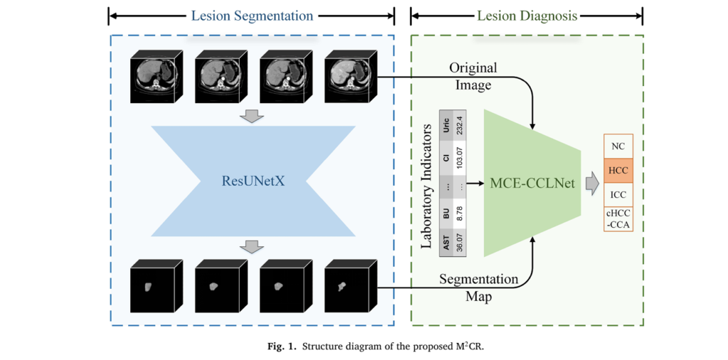
Developed by researchers at Chongqing University of Posts and Telecommunications and collaborating medical institutions, M2CR represents the first unified diagnostic framework capable of identifying all primary liver cancer subtypes through intelligent fusion of contrast-enhanced CT imaging and laboratory biomarkers. This article explores how this sophisticated system works, why it outperforms existing methods, and what it means for the future of precision oncology.
Understanding the Challenge: Why Liver Cancer Diagnosis Demands Innovation
The Complexity of Primary Liver Cancer Subtypes
Primary liver cancer isn’t a single disease—it’s a spectrum of malignancies with distinct origins, behaviors, and treatment protocols. Hepatocellular carcinoma arises from hepatocytes, the liver’s primary functional cells, and typically develops in cirrhotic livers. Intrahepatic cholangiocarcinoma originates from bile duct epithelial cells and often presents with different therapeutic sensitivities. The combined hepatocellular-cholangiocarcinoma represents a rare hybrid containing elements of both, making it particularly challenging to identify.
Traditional diagnostic workflows require radiologists to manually evaluate CT images across multiple enhancement phases while simultaneously interpreting laboratory values—a cognitively demanding process vulnerable to inter-observer variability. Studies demonstrate that diagnostic accuracy varies significantly based on radiologist experience, with subtle imaging features often missed in busy clinical environments.
Limitations of Current AI Approaches
While artificial intelligence has made inroads into medical imaging, most existing systems suffer from critical limitations:
- Single-modality dependency: Many models analyze only imaging data, ignoring valuable laboratory biomarkers that clinicians routinely use
- Incomplete subtype coverage: Prior AI systems focused exclusively on HCC detection, leaving ICC and cHCC-CCA undiagnosed
- Phase inflexibility: Conventional models assume complete four-phase CT studies, failing when clinical realities produce incomplete data
- Superficial fusion: Simple concatenation of imaging and clinical data fails to capture complex inter-modal relationships
M2CR Architecture: How Multimodal Intelligence Works
The Dual-Network Design
M2CR operates through two synergistic neural networks that mirror the clinical diagnostic process:
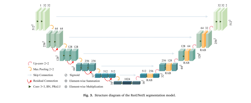
1. ResUNetX: Precision Lesion Segmentation
The system’s foundation lies in accurate tumor delineation. ResUNetX employs a sophisticated encoder-decoder architecture with five down-sampling and five up-sampling operations, enabling it to capture both coarse anatomical structures and fine lesion boundaries. What distinguishes this network is its Residual Attention Block (RAB) mechanism, which generates attention mappings across channel and spatial dimensions.
The mathematical formulation of the RAB operation follows:
\[ \mathbf{f}^{\prime} = \sigma\!\left( \mathrm{MLP}\!\left(\mathrm{AvgPool}(\mathbf{f})\right) + \mathrm{MLP}\!\left(\mathrm{MaxPool}(\mathbf{f})\right) \right) \] \[ \mathbf{f}^{\prime\prime} = \sigma\!\left( \mathrm{Conv}_{7 \times 7} \left( \left[ \mathrm{AvgPool}(\mathbf{f}^{\prime}); \mathrm{MaxPool}(\mathbf{f}^{\prime}) \right] \right) \right) + \mathrm{Conv}_{1 \times 1}(\mathbf{f}) \]Where σ represents the sigmoid activation function, and MLP(⋅) denotes multi-layer perceptron processing. This dual-attention approach guides the model to focus on diagnostically relevant regions while suppressing background interference.
Following segmentation, a Fully Connected Conditional Random Field (FC-CRF) refines boundaries by incorporating spatial context across three-dimensional volumes, addressing the limitation of slice-by-slice processing.
2. MCE-CCLNet: Intelligent Multimodal Classification
The Multimodal Cross-Attention with Coupled Contrastive Learning Network serves as M2CR’s diagnostic engine. This architecture processes four distinct data streams:
- Original CECT images across available phases
- Segmentation masks from ResUNetX (as structured imaging priors)
- Laboratory indicator values (10 key biomarkers)
- Phase index embeddings (handling variable phase availability)
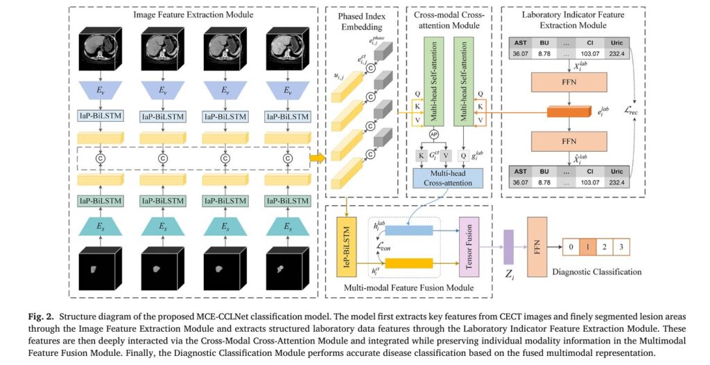
Handling Clinical Variability: The BiLSTM Solution
Real-world CT protocols vary enormously. Some patients have complete four-phase studies (plain, arterial, venous, delayed), while others present with incomplete data due to contrast allergies, hemodynamic instability, or resource constraints. M2CR addresses this through two specialized modules:
| Module | Function | Technical Implementation |
|---|---|---|
| IaP-BiLSTM | Intra-phase feature aggregation | Bidirectional LSTM processing slice sequences within single phases |
| IeP-BiLSTM | Inter-phase feature integration | Cross-phase BiLSTM combining information from available phases |
The intra-phase processing captures spatial relationships through:
\[ u_{i,j,N} = \mathrm{BiLSTM}\!\left( \left[ u_{i,j,1},\, u_{i,j,2},\, \ldots,\, u_{i,j,N_{i,j}} \right], \, h_{0} \right) \]Where Ni,j represents the slice count for patient i in phase j, accommodating variable layer thicknesses and scan ranges.
Phase index embedding uses learnable representations:
\[ e^{\text{phase}}_{i,j} = \mathrm{OneHot}(j)\,\cdot\, M \]This explicit phase encoding enables the model to understand enhancement timing patterns critical for characterizing tumor vascularity.
Cross-Modal Fusion: Where Imaging Meets Biochemistry
The Contrastive Learning Approach
A persistent challenge in multimodal AI is feature heterogeneity—imaging features and laboratory values occupy fundamentally different representation spaces. M2CR employs contrastive learning to align these modalities while preserving their distinctive information.
The contrastive loss function minimizes distance between matched imaging-laboratory pairs while maximizing separation from unmatched samples:
\[ L_{\text{con}} = \frac{1}{B} \sum_{i=1}^{B} \max\!\Big( 0,\; d\!\left(h_{i}^{ct},\, h_{i}^{lab}\right) – d\!\left(h_{i}^{ct},\, h_{i}^{\prime\,lab}\right) + \psi \Big) \]Here, d(⋅,⋅) measures cosine distance, B denotes batch size, and ψ = 0.1 serves as a margin parameter ensuring meaningful separation.
Tensor Fusion: Capturing Complex Interactions
Rather than simple concatenation, M2CR implements tensor fusion to model high-order interactions between modalities. The outer product operation creates a comprehensive interaction matrix:
\[ Z_i = \left[ h^{\mathrm{ict}}_{1} \right] \otimes \left[ h^{\mathrm{ilab}}_{1} \right] \]This formulation preserves unimodal features (through the constant 1 augmentation) while explicitly representing cross-modal relationships, yielding superior performance over mean, max, or concatenation alternatives.
Laboratory Feature Integrity Through Reconstruction
To ensure laboratory features maintain clinical interpretability, M2CR incorporates an autoencoder-style reconstruction pathway:
\[ L_{\text{rec}} = \sum_{i=1}^{D_{\text{lab}}} \left( X_{i}^{\text{lab}} – \hat{X}_{i}^{\text{lab}} \right)^{2} \]Where Dlab = 10 represents the selected biomarker panel. This reconstruction constraint prevents the network from generating abstract, uninterpretable laboratory representations.
Performance Validation: Clinical Evidence
Internal Dataset Results
M2CR was validated on a comprehensive dataset comprising 361 subjects across four medical centers:
- 83 normal controls
- 94 hepatocellular carcinoma cases
- 99 intrahepatic cholangiocarcinoma cases
- 85 combined hepatocellular-cholangiocarcinoma cases
Each case included four-phase CECT with pathological confirmation, yielding 152,964 annotated slices.
Diagnostic Performance Metrics:
| Metric | Value | Confidence Interval |
|---|---|---|
| Macro-average Accuracy | 0.97 | (0.93, 1.00) |
| Macro-average F1-Score | 0.93 | (0.86, 0.98) |
| Macro-average AUROC | 0.96 | (0.92, 0.99) |
| Macro-average AUPRC | 0.89 | (0.86, 0.99) |
Notably, the system achieved perfect classification for normal controls and HCC cases, with slightly reduced but still excellent performance on ICC (AUROC 0.87) reflecting that subtype’s inherent diagnostic complexity.
Segmentation Excellence
ResUNetX demonstrated superior tumor delineation compared to established architectures:
- HCC segmentation: Dice coefficient 0.8219 (arterial phase)
- ICC segmentation: Dice coefficient 0.8153 (arterial phase)
- cHCC-CCA segmentation: Dice coefficient 0.8559 (venous phase)
These values significantly outperformed U-Net, U-Net++, FCN, and even the Segment Anything Model (SAM) adapted for medical imaging, validating the specialized architectural choices.
Robustness to Incomplete Data
A critical real-world test evaluated performance across varying phase availability. M2CR maintained strong diagnostic capability even with limited imaging:
- Single-phase performance: AUROC 0.75–0.82 depending on phase
- Two-phase combinations: AUROC 0.81–0.88
- Three-phase combinations: AUROC 0.86–0.91
- Complete four-phase: AUROC 0.96
Crucially, the multimodal advantage was consistent across all combinations—the laboratory data provided complementary information that compensated for missing imaging phases.
External Validation and Generalization
To assess cross-institutional reliability, researchers conducted leave-one-hospital-out cross-validation. Performance remained robust:
- Accuracy: 0.86 (0.77, 0.93)
- F1-Score: 0.85 (0.76, 0.93)
- AUROC: 0.91 (0.84, 0.97)
This demonstrates M2CR’s potential for deployment across diverse healthcare environments without institution-specific retraining.
Clinical Implementation: From Algorithm to Bedside
Real-World Deployment Experience
Between December 2023 and February 2024, M2CR underwent prospective evaluation at Chongqing Yubei District People’s Hospital. The system integrated with existing Laboratory Information Systems (LIS) and Picture Archiving and Communication Systems (PACS), automatically retrieving relevant data for newly imaged patients.
Key implementation features included:
- Automated data pipeline: Direct API connections to hospital information systems
- Interactive visualization: Side-by-side display of original images, segmentation overlays, and probability scores
- Phase-agnostic processing: Graceful handling of incomplete studies without user intervention
- Diagnostic confidence scoring: Transparent probability outputs for HCC, ICC, cHCC-CCA, and normal liver
During this pilot, the system generated predictions for 24 consecutive cases. Clinical review found:
- 22/24 cases (91.7%) showed concordance with expert radiologist assessment
- 12 patients proceeded to treatment, with pathological confirmation matching M2CR predictions in 10/12 cases
- 2 discordant cases were ultimately identified as benign hemangiomas, highlighting the system’s conservative bias toward malignancy detection
Critical Laboratory Biomarkers
Analysis revealed the ten most diagnostically valuable laboratory indicators:
- Red Cell Distribution Width (RDW)
- Age (demographic/clinical factor)
- Cholinesterase
- Alpha-Fetoprotein (AFP)
- Hematocrit
- Carcinoembryonic Antigen (CEA)
- Mean Platelet Volume
- Aspartate Aminotransferase (AST)
- Indirect Bilirubin
- Plateletcrit
Notably, traditional markers like AFP ranked fourth in importance, while hematological parameters (RDW, platelet indices) demonstrated unexpected diagnostic value—insights that emerged from the data-driven feature selection process rather than conventional clinical assumptions.
Technical Innovations and Their Significance
Addressing Modality Heterogeneity
The contrastive-tensor fusion combination represents a methodological advance over existing multimodal strategies:
- Early fusion (direct concatenation): Fails to model complex interactions
- Late fusion (decision-level combination): Loses fine-grained feature relationships
- Intermediate fusion (MCE-CCLNet approach): Balances alignment and specificity
Ablation studies confirmed each component’s contribution:
| Component Addition | Accuracy Improvement | Key Benefit |
|---|---|---|
| Baseline (imaging only) | — | Reference standard |
| + Phase Index Embedding | +0% | Temporal structure awareness |
| + Segmentation Masks | +1% | Lesion-focused attention |
| + Reconstruction Loss | +2% | Feature distribution preservation |
| + Contrastive Loss | +2% | Cross-modal alignment |
Training Efficiency
The hybrid DC loss function (combining Dice and improved cross-entropy losses) accelerated convergence during ResUNetX training:
\[ L_{\mathrm{DC}} = \varepsilon\, L_{\mathrm{Dice}} + \left(1 – \varepsilon\right) L_{\mathrm{ICE}} \]With ε = 0.5 providing optimal balance, training loss stabilized 40% faster than conventional cross-entropy alone, reaching superior final performance.
Implications for Precision Oncology
Transforming Diagnostic Workflows
M2CR’s clinical value extends beyond accuracy metrics:
- Standardization: Reduces inter-observer variability in heterogeneous imaging environments
- Efficiency: Automated preprocessing and inference accelerate reporting
- Completeness: Systematic evaluation of all primary liver cancer subtypes prevents diagnostic omission
- Accessibility: Decision support enables consistent quality across experience levels
Future Development Trajectories
The modular architecture supports several expansion pathways:
- Genomic integration: Incorporating molecular profiling data for precision treatment matching
- Longitudinal analysis: Tracking treatment response through sequential imaging
- Multi-organ assessment: Extending to metastatic disease evaluation
- Prognostic modeling: Predicting survival and recurrence beyond diagnosis
Conclusion: A New Paradigm for Intelligent Diagnosis
M2CR exemplifies how artificial intelligence can transcend simple pattern recognition to emulate sophisticated clinical reasoning. By architecturally mirroring how expert physicians integrate diverse information sources—imaging morphology, enhancement dynamics, biochemical markers, and clinical context—this system achieves both high accuracy and clinical interpretability.
The key innovations—variable-phase handling through specialized BiLSTM modules, contrastive alignment of heterogeneous data types, and tensor-based fusion preserving unimodal characteristics—address fundamental challenges that have limited prior multimodal medical AI systems.
For clinicians and healthcare administrators, M2CR offers a validated, deployment-ready solution for enhancing liver cancer diagnostic accuracy. For researchers, it provides a methodological template for multimodal medical AI development. For patients, it promises more reliable, efficient pathways to accurate diagnosis and appropriate treatment.
Have you encountered challenges with liver lesion characterization in your practice or research? Share your experiences with multimodal diagnostic approaches in the comments below. For those interested in implementing AI-assisted diagnostic systems, what technical or clinical barriers do you foresee? Subscribe to our updates for continued coverage of advances in medical artificial intelligence and precision oncology.
Below is the comprehensive implementation of the M2CR system based on the research paper. This will include the complete ResUNetX segmentation model and MCE-CCLNet classification model with all the described components.
"""
M2CR: Multimodal Multitask Collaborative Reasoning for Primary Liver Cancer Diagnosis
Complete PyTorch Implementation
Based on: Huang et al., Expert Systems With Applications, 2026
"""
import torch
import torch.nn as nn
import torch.nn.functional as F
import math
from typing import List, Tuple, Optional, Dict
from collections import OrderedDict
# ============================================================================
# PART 1: ResUNetX - Lesion Segmentation Network
# ============================================================================
class ResidualAttentionBlock(nn.Module):
"""
Residual Attention Block (RAB) for ResUNetX
Implements channel and spatial attention mechanisms
"""
def __init__(self, channels: int, reduction: int = 16):
super().__init__()
self.channels = channels
# Channel attention components
self.avg_pool = nn.AdaptiveAvgPool2d(1)
self.max_pool = nn.AdaptiveMaxPool2d(1)
self.mlp = nn.Sequential(
nn.Linear(channels, channels // reduction, bias=False),
nn.ReLU(inplace=True),
nn.Linear(channels // reduction, channels, bias=False)
)
# Spatial attention components
self.conv_spatial = nn.Conv2d(2, 1, kernel_size=7, padding=3, bias=False)
self.conv_residual = nn.Conv2d(channels, channels, kernel_size=1, bias=False)
self.sigmoid = nn.Sigmoid()
def forward(self, x: torch.Tensor) -> torch.Tensor:
# Channel attention
avg_out = self.mlp(self.avg_pool(x).view(x.size(0), -1))
max_out = self.mlp(self.max_pool(x).view(x.size(0), -1))
channel_att = self.sigmoid(avg_out + max_out).view(x.size(0), self.channels, 1, 1)
# Spatial attention
avg_spatial = torch.mean(x, dim=1, keepdim=True)
max_spatial, _ = torch.max(x, dim=1, keepdim=True)
spatial_concat = torch.cat([avg_spatial, max_spatial], dim=1)
spatial_att = self.sigmoid(self.conv_spatial(spatial_concat))
# Apply attention
x_attended = x * channel_att * spatial_att
# Residual connection
residual = self.conv_residual(x)
return x_attended + residual
class EncoderBlock(nn.Module):
"""Encoder block with convolution, batch norm, PReLU, and optional RAB"""
def __init__(self, in_ch: int, out_ch: int, use_rab: bool = False):
super().__init__()
self.conv = nn.Sequential(
nn.Conv2d(in_ch, out_ch, kernel_size=3, padding=1, bias=False),
nn.BatchNorm2d(out_ch),
nn.PReLU(out_ch)
)
self.use_rab = use_rab
if use_rab:
self.rab = ResidualAttentionBlock(out_ch)
def forward(self, x: torch.Tensor) -> torch.Tensor:
x = self.conv(x)
if self.use_rab:
x = self.rab(x)
return x
class DecoderBlock(nn.Module):
"""Decoder block with upsampling, concatenation, and convolution"""
def __init__(self, in_ch: int, out_ch: int, use_rab: bool = False):
super().__init__()
self.upconv = nn.ConvTranspose2d(in_ch, out_ch, kernel_size=2, stride=2)
self.conv = nn.Sequential(
nn.Conv2d(in_ch, out_ch, kernel_size=3, padding=1, bias=False),
nn.BatchNorm2d(out_ch),
nn.PReLU(out_ch),
nn.Conv2d(out_ch, out_ch, kernel_size=3, padding=1, bias=False),
nn.BatchNorm2d(out_ch),
nn.PReLU(out_ch)
)
self.use_rab = use_rab
if use_rab:
self.rab = ResidualAttentionBlock(out_ch)
def forward(self, x: torch.Tensor, skip: torch.Tensor) -> torch.Tensor:
x = self.upconv(x)
# Handle size mismatch
if x.size() != skip.size():
x = F.interpolate(x, size=skip.shape[2:], mode='bilinear', align_corners=True)
x = torch.cat([x, skip], dim=1)
x = self.conv(x)
if self.use_rab:
x = self.rab(x)
return x
class ResUNetX(nn.Module):
"""
ResUNetX: Residual U-Net with Attention for Liver Lesion Segmentation
Architecture: 5-level encoder-decoder with residual connections and RAB modules
"""
def __init__(
self,
in_channels: int = 1,
num_classes: int = 2, # Background + Lesion
base_channels: int = 32,
dropout: float = 0.1
):
super().__init__()
# Encoder path (5 levels)
self.enc1 = EncoderBlock(in_channels, base_channels, use_rab=False)
self.enc2 = EncoderBlock(base_channels, base_channels * 2, use_rab=False)
self.enc3 = EncoderBlock(base_channels * 2, base_channels * 4, use_rab=False)
self.enc4 = EncoderBlock(base_channels * 4, base_channels * 8, use_rab=False)
self.enc5 = EncoderBlock(base_channels * 8, base_channels * 16, use_rab=False)
self.pool = nn.MaxPool2d(2, 2)
# Decoder path with RAB in first 4 decoders
self.dec4 = DecoderBlock(base_channels * 16, base_channels * 8, use_rab=True)
self.dec3 = DecoderBlock(base_channels * 8, base_channels * 4, use_rab=True)
self.dec2 = DecoderBlock(base_channels * 4, base_channels * 2, use_rab=True)
self.dec1 = DecoderBlock(base_channels * 2, base_channels, use_rab=True)
# Final convolution
self.final = nn.Conv2d(base_channels, num_classes, kernel_size=1)
# Dropout
self.dropout = nn.Dropout2d(dropout) if dropout > 0 else nn.Identity()
self._initialize_weights()
def _initialize_weights(self):
for m in self.modules():
if isinstance(m, nn.Conv2d) or isinstance(m, nn.ConvTranspose2d):
nn.init.kaiming_normal_(m.weight, mode='fan_out', nonlinearity='relu')
elif isinstance(m, nn.BatchNorm2d):
nn.init.constant_(m.weight, 1)
nn.init.constant_(m.bias, 0)
def forward(self, x: torch.Tensor) -> torch.Tensor:
# Store input size for potential resizing
input_size = x.shape[2:]
# Encoder path
e1 = self.enc1(x)
e2 = self.enc2(self.pool(e1))
e3 = self.enc3(self.pool(e2))
e4 = self.enc4(self.pool(e3))
e5 = self.enc5(self.pool(e4))
e5 = self.dropout(e5)
# Decoder path with skip connections
d4 = self.dec4(e5, e4)
d3 = self.dec3(d4, e3)
d2 = self.dec2(d3, e2)
d1 = self.dec1(d2, e1)
# Final output
out = self.final(d1)
# Resize to input size if needed
if out.shape[2:] != input_size:
out = F.interpolate(out, size=input_size, mode='bilinear', align_corners=True)
return out
# ============================================================================
# PART 2: Hybrid Loss Functions for Segmentation
# ============================================================================
class DiceLoss(nn.Module):
"""Dice loss for segmentation with smoothing"""
def __init__(self, smooth: float = 1e-5):
super().__init__()
self.smooth = smooth
def forward(self, pred: torch.Tensor, target: torch.Tensor) -> torch.Tensor:
pred = F.softmax(pred, dim=1)
# One-hot encode target if needed
if target.dim() == 3 or (target.dim() == 4 and target.size(1) == 1):
target = F.one_hot(target.long(), num_classes=pred.size(1))
target = target.permute(0, 3, 1, 2).float()
# Flatten
pred = pred.view(pred.size(0), pred.size(1), -1)
target = target.view(target.size(0), target.size(1), -1)
intersection = (pred * target).sum(dim=2)
union = pred.sum(dim=2) + target.sum(dim=2)
dice = (2.0 * intersection + self.smooth) / (union + self.smooth)
return 1.0 - dice.mean()
class ImprovedCrossEntropyLoss(nn.Module):
"""Weighted cross-entropy loss handling class imbalance"""
def __init__(self, weights: Optional[torch.Tensor] = None):
super().__init__()
self.weights = weights
def forward(self, pred: torch.Tensor, target: torch.Tensor) -> torch.Tensor:
if target.dim() == 4:
target = target.squeeze(1)
return F.cross_entropy(pred, target.long(), weight=self.weights)
class DCLoss(nn.Module):
"""
DC Loss: Hybrid Dice + Improved Cross-Entropy Loss
L_DC = ε * L_Dice + (1 - ε) * L_ICE
"""
def __init__(self, epsilon: float = 0.5, class_weights: Optional[torch.Tensor] = None):
super().__init__()
self.epsilon = epsilon
self.dice_loss = DiceLoss()
self.ce_loss = ImprovedCrossEntropyLoss(weights=class_weights)
def forward(self, pred: torch.Tensor, target: torch.Tensor) -> torch.Tensor:
dice = self.dice_loss(pred, target)
ce = self.ce_loss(pred, target)
return self.epsilon * dice + (1.0 - self.epsilon) * ce
# ============================================================================
# PART 3: FC-CRF Post-Processing (Simplified Implementation)
# ============================================================================
class FullyConnectedCRF(nn.Module):
"""
Simplified Fully Connected CRF for post-processing
(Full implementation would require densecrf library)
"""
def __init__(self, num_iterations: int = 5, gaussian_sigma: float = 3.0):
super().__init__()
self.num_iterations = num_iterations
self.gaussian_sigma = gaussian_sigma
def forward(self, logits: torch.Tensor, image: torch.Tensor) -> torch.Tensor:
"""
Simplified CRF inference - in practice, use pydensecrf or similar
This is a placeholder for the bilateral filtering operation
"""
# Apply Gaussian smoothing as approximation
probs = F.softmax(logits, dim=1)
# Simple Gaussian filter
kernel_size = int(6 * self.gaussian_sigma) | 1 # Make odd
if kernel_size < 3:
kernel_size = 3
padding = kernel_size // 2
sigma = self.gaussian_sigma
# Create Gaussian kernel
x_coord = torch.arange(kernel_size, dtype=torch.float32, device=logits.device)
gaussian_kernel = torch.exp(-(x_coord - padding) ** 2 / (2 * sigma ** 2))
gaussian_kernel = gaussian_kernel / gaussian_kernel.sum()
# 2D Gaussian
kernel_2d = gaussian_kernel.unsqueeze(0) * gaussian_kernel.unsqueeze(1)
kernel_2d = kernel_2d / kernel_2d.sum()
# Apply to each class
smoothed = []
for c in range(probs.size(1)):
channel = probs[:, c:c+1, :, :]
smoothed_c = F.conv2d(
channel,
kernel_2d.view(1, 1, kernel_size, kernel_size).to(logits.device),
padding=padding
)
smoothed.append(smoothed_c)
smoothed_probs = torch.cat(smoothed, dim=1)
# Convert back to logits
return torch.log(smoothed_probs + 1e-8)
# ============================================================================
# PART 4: MCE-CCLNet - Multimodal Classification Network
# ============================================================================
class PhaseIndexEmbedding(nn.Module):
"""Learnable embedding for CT phase indices (0-3 for PP, AP, VP, DP)"""
def __init__(self, num_phases: int = 4, embed_dim: int = 128):
super().__init__()
self.embedding = nn.Embedding(num_phases, embed_dim)
def forward(self, phase_indices: torch.Tensor) -> torch.Tensor:
"""
Args:
phase_indices: (batch_size, num_phases) or (batch_size,)
indicating which phases are present
Returns:
embedded: (batch_size, num_phases, embed_dim) or (batch_size, embed_dim)
"""
return self.embedding(phase_indices)
class ResNetFeatureExtractor(nn.Module):
"""Simplified ResNet backbone for CT feature extraction"""
def __init__(self, in_channels: int = 1, pretrained: bool = False):
super().__init__()
# Initial conv
self.conv1 = nn.Conv2d(in_channels, 64, kernel_size=7, stride=2, padding=3, bias=False)
self.bn1 = nn.BatchNorm2d(64)
self.relu = nn.ReLU(inplace=True)
self.maxpool = nn.MaxPool2d(kernel_size=3, stride=2, padding=1)
# Residual layers (simplified)
self.layer1 = self._make_layer(64, 64, 2, stride=1)
self.layer2 = self._make_layer(64, 128, 2, stride=2)
self.layer3 = self._make_layer(128, 256, 2, stride=2)
self.layer4 = self._make_layer(256, 512, 2, stride=2)
self.avgpool = nn.AdaptiveAvgPool2d((1, 1))
self.feature_dim = 512
def _make_layer(self, in_ch: int, out_ch: int, num_blocks: int, stride: int):
layers = []
# First block with downsampling
layers.append(nn.Conv2d(in_ch, out_ch, 3, stride=stride, padding=1, bias=False))
layers.append(nn.BatchNorm2d(out_ch))
layers.append(nn.ReLU(inplace=True))
layers.append(nn.Conv2d(out_ch, out_ch, 3, padding=1, bias=False))
layers.append(nn.BatchNorm2d(out_ch))
# Shortcut
if stride != 1 or in_ch != out_ch:
shortcut = nn.Sequential(
nn.Conv2d(in_ch, out_ch, 1, stride=stride, bias=False),
nn.BatchNorm2d(out_ch)
)
else:
shortcut = nn.Identity()
layers.append(shortcut)
layers.append(nn.ReLU(inplace=True))
# Remaining blocks
for _ in range(num_blocks - 1):
layers.append(nn.Conv2d(out_ch, out_ch, 3, padding=1, bias=False))
layers.append(nn.BatchNorm2d(out_ch))
layers.append(nn.ReLU(inplace=True))
layers.append(nn.Conv2d(out_ch, out_ch, 3, padding=1, bias=False))
layers.append(nn.BatchNorm2d(out_ch))
layers.append(nn.Identity()) # Shortcut
layers.append(nn.ReLU(inplace=True))
return nn.Sequential(*layers)
def forward(self, x: torch.Tensor) -> torch.Tensor:
x = self.conv1(x)
x = self.bn1(x)
x = self.relu(x)
x = self.maxpool(x)
x = self.layer1(x)
x = self.layer2(x)
x = self.layer3(x)
x = self.layer4(x)
x = self.avgpool(x)
x = torch.flatten(x, 1)
return x
class IntraPhaseBiLSTM(nn.Module):
"""
IaP-BiLSTM: Handles variable slice counts within a single phase
Processes 3D volume as sequence of 2D slices
"""
def __init__(
self,
input_dim: int = 512,
hidden_dim: int = 256,
num_layers: int = 2,
dropout: float = 0.3
):
super().__init__()
self.hidden_dim = hidden_dim
self.bilstm = nn.LSTM(
input_size=input_dim,
hidden_size=hidden_dim,
num_layers=num_layers,
batch_first=True,
bidirectional=True,
dropout=dropout if num_layers > 1 else 0
)
# Output dimension is 2 * hidden_dim (bidirectional)
self.output_dim = hidden_dim * 2
def forward(self, slice_features: torch.Tensor) -> torch.Tensor:
"""
Args:
slice_features: (batch, num_slices, feature_dim)
Returns:
phase_feature: (batch, output_dim) - aggregated phase representation
"""
# Pack if variable lengths (handled by padding in practice)
lstm_out, (hidden, cell) = self.bilstm(slice_features)
# Use final hidden state (concatenated forward/backward)
# hidden: (num_layers * 2, batch, hidden_dim)
forward_h = hidden[-2, :, :] # Last layer forward
backward_h = hidden[-1, :, :] # Last layer backward
phase_feature = torch.cat([forward_h, backward_h], dim=1)
return phase_feature
class InterPhaseBiLSTM(nn.Module):
"""
IeP-BiLSTM: Aggregates features across multiple phases
Handles variable phase combinations
"""
def __init__(
self,
input_dim: int = 512, # After concatenation with phase embedding
hidden_dim: int = 256,
num_layers: int = 2,
dropout: float = 0.3
):
super().__init__()
self.bilstm = nn.LSTM(
input_size=input_dim,
hidden_size=hidden_dim,
num_layers=num_layers,
batch_first=True,
bidirectional=True,
dropout=dropout if num_layers > 1 else 0
)
self.output_dim = hidden_dim * 2
def forward(self, phase_features: torch.Tensor, phase_mask: Optional[torch.Tensor] = None) -> torch.Tensor:
"""
Args:
phase_features: (batch, max_phases, feature_dim)
phase_mask: (batch, max_phases) boolean mask for valid phases
Returns:
aggregated: (batch, output_dim)
"""
lstm_out, (hidden, cell) = self.bilstm(phase_features)
forward_h = hidden[-2, :, :]
backward_h = hidden[-1, :, :]
aggregated = torch.cat([forward_h, backward_h], dim=1)
return aggregated
class LaboratoryFeatureExtractor(nn.Module):
"""
FFN-based laboratory indicator feature extraction with reconstruction
"""
def __init__(
self,
num_indicators: int = 10,
hidden_dims: List[int] = [128, 256],
embed_dim: int = 128,
dropout: float = 0.3
):
super().__init__()
# Encoder
encoder_layers = []
prev_dim = num_indicators
for h_dim in hidden_dims:
encoder_layers.extend([
nn.Linear(prev_dim, h_dim),
nn.BatchNorm1d(h_dim),
nn.PReLU(),
nn.Dropout(dropout)
])
prev_dim = h_dim
encoder_layers.append(nn.Linear(prev_dim, embed_dim))
self.encoder = nn.Sequential(*encoder_layers)
# Decoder for reconstruction loss
decoder_layers = []
prev_dim = embed_dim
for h_dim in reversed(hidden_dims):
decoder_layers.extend([
nn.Linear(prev_dim, h_dim),
nn.PReLU()
])
prev_dim = h_dim
decoder_layers.append(nn.Linear(prev_dim, num_indicators))
self.decoder = nn.Sequential(*decoder_layers)
self.embed_dim = embed_dim
def forward(self, x: torch.Tensor) -> Tuple[torch.Tensor, torch.Tensor]:
"""
Returns:
encoded: Laboratory feature embedding
reconstructed: Reconstructed input for L_rec computation
"""
encoded = self.encoder(x)
reconstructed = self.decoder(encoded)
return encoded, reconstructed
class MultiHeadCrossAttention(nn.Module):
"""Multi-head cross-attention for modality interaction"""
def __init__(self, dim: int, num_heads: int = 8, dropout: float = 0.1):
super().__init__()
assert dim % num_heads == 0, "dim must be divisible by num_heads"
self.dim = dim
self.num_heads = num_heads
self.head_dim = dim // num_heads
self.scale = self.head_dim ** -0.5
self.q_proj = nn.Linear(dim, dim)
self.k_proj = nn.Linear(dim, dim)
self.v_proj = nn.Linear(dim, dim)
self.out_proj = nn.Linear(dim, dim)
self.dropout = nn.Dropout(dropout)
def forward(
self,
query: torch.Tensor,
key: torch.Tensor,
value: torch.Tensor,
mask: Optional[torch.Tensor] = None
) -> torch.Tensor:
batch_size = query.size(0)
# Project and reshape
Q = self.q_proj(query).view(batch_size, -1, self.num_heads, self.head_dim).transpose(1, 2)
K = self.k_proj(key).view(batch_size, -1, self.num_heads, self.head_dim).transpose(1, 2)
V = self.v_proj(value).view(batch_size, -1, self.num_heads, self.head_dim).transpose(1, 2)
# Attention
scores = torch.matmul(Q, K.transpose(-2, -1)) * self.scale
if mask is not None:
scores = scores.masked_fill(mask == 0, float('-inf'))
attn = F.softmax(scores, dim=-1)
attn = self.dropout(attn)
out = torch.matmul(attn, V)
out = out.transpose(1, 2).contiguous().view(batch_size, -1, self.dim)
out = self.out_proj(out)
return out
class CrossModalAttentionModule(nn.Module):
"""
Cross-modal cross-attention between imaging and laboratory features
"""
def __init__(
self,
ct_dim: int = 512,
lab_dim: int = 128,
num_heads: int = 8,
dropout: float = 0.1
):
super().__init__()
# Self-attention for each modality
self.ct_self_attn = MultiHeadCrossAttention(ct_dim, num_heads, dropout)
self.lab_self_attn = MultiHeadCrossAttention(lab_dim, num_heads, dropout)
# Cross-attention: lab queries CT
self.cross_attn = MultiHeadCrossAttention(lab_dim, num_heads, dropout)
# Projection to common dimension if needed
self.ct_to_lab = nn.Linear(ct_dim, lab_dim) if ct_dim != lab_dim else nn.Identity()
self.norm1 = nn.LayerNorm(ct_dim)
self.norm2 = nn.LayerNorm(lab_dim)
self.norm3 = nn.LayerNorm(lab_dim)
def forward(
self,
ct_features: torch.Tensor, # (batch, num_patches, ct_dim)
lab_features: torch.Tensor # (batch, lab_dim) -> (batch, 1, lab_dim)
) -> Tuple[torch.Tensor, torch.Tensor]:
# Add sequence dimension to lab if needed
if lab_features.dim() == 2:
lab_features = lab_features.unsqueeze(1)
# Self-attention
ct_attended = self.ct_self_attn(ct_features, ct_features, ct_features)
ct_attended = self.norm1(ct_attended + ct_features)
lab_attended = self.lab_self_attn(lab_features, lab_features, lab_features)
lab_attended = self.norm2(lab_attended + lab_features)
# Cross-attention: lab queries CT
ct_projected = self.ct_to_lab(ct_attended)
lab_cross = self.cross_attn(lab_attended, ct_projected, ct_projected)
lab_cross = self.norm3(lab_cross + lab_attended)
# Pool CT features
ct_pooled = ct_attended.mean(dim=1) # Global average pooling
return ct_pooled, lab_cross.squeeze(1)
class TensorFusion(nn.Module):
"""
Tensor fusion: outer product of extended feature vectors
Z = [h_ct; 1] ⊗ [h_lab; 1]
"""
def __init__(self, ct_dim: int, lab_dim: int):
super().__init__()
self.ct_dim = ct_dim
self.lab_dim = lab_dim
self.output_dim = (ct_dim + 1) * (lab_dim + 1)
def forward(self, ct_feat: torch.Tensor, lab_feat: torch.Tensor) -> torch.Tensor:
batch_size = ct_feat.size(0)
# Extend with constant 1
ct_extended = torch.cat([ct_feat, torch.ones(batch_size, 1, device=ct_feat.device)], dim=1)
lab_extended = torch.cat([lab_feat, torch.ones(batch_size, 1, device=lab_feat.device)], dim=1)
# Outer product
# ct_extended: (B, ct_dim+1), lab_extended: (B, lab_dim+1)
# Result: (B, ct_dim+1, lab_dim+1)
fusion = torch.bmm(ct_extended.unsqueeze(2), lab_extended.unsqueeze(1))
# Flatten
fusion = fusion.view(batch_size, -1)
return fusion
class ContrastiveLoss(nn.Module):
"""
Contrastive loss for cross-modal alignment
L_con = max(0, d(h_ct, h_lab) - d(h_ct, h_lab') + ψ)
"""
def __init__(self, margin: float = 0.1):
super().__init__()
self.margin = margin
def forward(
self,
ct_features: torch.Tensor,
lab_features: torch.Tensor
) -> torch.Tensor:
batch_size = ct_features.size(0)
# Normalize features
ct_norm = F.normalize(ct_features, p=2, dim=1)
lab_norm = F.normalize(lab_features, p=2, dim=1)
# Compute cosine distances
# Positive pairs (same sample)
pos_dist = 1 - (ct_norm * lab_norm).sum(dim=1) # (B,)
# Negative pairs (different samples)
# Compute all pairwise distances
# ct_norm: (B, D), lab_norm: (B, D)
# sim_matrix: (B, B)
sim_matrix = torch.mm(ct_norm, lab_norm.t())
neg_dist = 1 - sim_matrix # (B, B)
# For each sample, hardest negative (excluding self)
mask = torch.eye(batch_size, device=ct_features.device).bool()
neg_dist_masked = neg_dist.masked_fill(mask, float('inf'))
hardest_neg = neg_dist_masked.min(dim=1)[0]
# Contrastive loss
loss = torch.clamp(pos_dist - hardest_neg + self.margin, min=0.0)
return loss.mean()
class MCE_CCLNet(nn.Module):
"""
MCE-CCLNet: Multimodal Cross-Attention with Coupled Contrastive Learning Network
Main classification network for primary liver cancer diagnosis
"""
def __init__(
self,
num_classes: int = 4, # NC, HCC, ICC, cHCC-CCA
num_phases: int = 4,
num_lab_indicators: int = 10,
ct_feature_dim: int = 512,
lab_embed_dim: int = 128,
lstm_hidden: int = 256,
num_attention_heads: int = 8,
dropout: float = 0.3
):
super().__init__()
self.num_classes = num_classes
self.num_phases = num_phases
# Image feature extractors (shared weights for original and segmented)
self.image_encoder = ResNetFeatureExtractor(in_channels=1)
self.seg_encoder = ResNetFeatureExtractor(in_channels=1)
# Phase index embedding
self.phase_embed = PhaseIndexEmbedding(num_phases, embed_dim=64)
# Intra-phase BiLSTM (per phase)
self.iap_bilstm = IntraPhaseBiLSTM(
input_dim=ct_feature_dim * 2, # Original + Segmented concatenated
hidden_dim=lstm_hidden,
dropout=dropout
)
# Inter-phase BiLSTM
iep_input_dim = self.iap_bilstm.output_dim + 64 # + phase embedding
self.iep_bilstm = InterPhaseBiLSTM(
input_dim=iep_input_dim,
hidden_dim=lstm_hidden,
dropout=dropout
)
# Laboratory feature extraction
self.lab_extractor = LaboratoryFeatureExtractor(
num_indicators=num_lab_indicators,
embed_dim=lab_embed_dim,
dropout=dropout
)
# Cross-modal attention
self.cross_modal_attn = CrossModalAttentionModule(
ct_dim=self.iep_bilstm.output_dim,
lab_dim=lab_embed_dim,
num_heads=num_attention_heads,
dropout=dropout
)
# Tensor fusion
self.tensor_fusion = TensorFusion(
ct_dim=self.iep_bilstm.output_dim,
lab_dim=lab_embed_dim
)
# Final classifier
fusion_dim = self.tensor_fusion.output_dim
self.classifier = nn.Sequential(
nn.Linear(fusion_dim, 512),
nn.LayerNorm(512),
nn.ReLU(inplace=True),
nn.Dropout(dropout),
nn.Linear(512, 256),
nn.LayerNorm(256),
nn.ReLU(inplace=True),
nn.Dropout(dropout),
nn.Linear(256, num_classes)
)
self._initialize_weights()
def _initialize_weights(self):
for m in self.modules():
if isinstance(m, nn.Linear):
nn.init.xavier_uniform_(m.weight)
if m.bias is not None:
nn.init.constant_(m.bias, 0)
def extract_phase_features(
self,
phase_images: torch.Tensor, # (B, N_slices, H, W)
phase_masks: torch.Tensor, # (B, N_slices, H, W)
phase_idx: int
) -> torch.Tensor:
"""
Extract features for a single phase using IaP-BiLSTM
"""
batch_size, num_slices = phase_images.size(0), phase_images.size(1)
# Process each slice
slice_features = []
for i in range(num_slices):
img_slice = phase_images[:, i:i+1, :, :] # (B, 1, H, W)
mask_slice = phase_masks[:, i:i+1, :, :] # (B, 1, H, W)
img_feat = self.image_encoder(img_slice) # (B, 512)
mask_feat = self.seg_encoder(mask_slice) # (B, 512)
combined = torch.cat([img_feat, mask_feat], dim=1) # (B, 1024)
slice_features.append(combined)
# Stack and process with BiLSTM
slice_features = torch.stack(slice_features, dim=1) # (B, N_slices, 1024)
phase_feature = self.iap_bilstm(slice_features) # (B, 512)
# Add phase embedding
phase_emb = self.phase_embed(
torch.tensor([phase_idx], device=phase_images.device)
).expand(batch_size, -1) # (B, 64)
return torch.cat([phase_feature, phase_emb], dim=1) # (B, 576)
def forward(
self,
images: Dict[str, torch.Tensor], # {'PP': (B, N, H, W), 'AP': ..., ...}
masks: Dict[str, torch.Tensor], # Segmentation masks same structure
lab_values: torch.Tensor, # (B, num_indicators)
available_phases: List[str] = None
) -> Dict[str, torch.Tensor]:
"""
Forward pass with variable phase handling
Args:
images: Dictionary mapping phase names to image tensors
masks: Dictionary mapping phase names to mask tensors
lab_values: Laboratory indicator values
available_phases: List of phase names present (e.g., ['AP', 'VP'])
"""
if available_phases is None:
available_phases = list(images.keys())
batch_size = lab_values.size(0)
device = lab_values.device
# Extract features for each available phase
phase_features_list = []
phase_order = ['PP', 'AP', 'VP', 'DP'] # Fixed order
for phase_name in available_phases:
if phase_name not in images:
continue
phase_idx = phase_order.index(phase_name)
phase_img = images[phase_name]
phase_mask = masks.get(phase_name, torch.zeros_like(phase_img))
# Pad or truncate to consistent slice count
if phase_img.size(1) > 32: # Max 32 slices
phase_img = phase_img[:, :32, :, :]
phase_mask = phase_mask[:, :32, :, :]
phase_feat = self.extract_phase_features(
phase_img, phase_mask, phase_idx
)
phase_features_list.append(phase_feat)
# Stack phases and apply IeP-BiLSTM
# Pad to fixed phase count if needed
max_phases = self.num_phases
num_present = len(phase_features_list)
if num_present == 0:
raise ValueError("At least one phase must be provided")
# Create padded tensor and mask
phase_tensor = torch.zeros(
batch_size, max_phases, phase_features_list[0].size(1),
device=device
)
phase_mask = torch.zeros(batch_size, max_phases, dtype=torch.bool, device=device)
for i, feat in enumerate(phase_features_list):
phase_tensor[:, i, :] = feat
phase_mask[:, i] = True
# Inter-phase aggregation
ct_aggregated = self.iep_bilstm(phase_tensor, phase_mask) # (B, 512)
# Laboratory features
lab_encoded, lab_reconstructed = self.lab_extractor(lab_values) # (B, 128)
# Cross-modal attention
# Reshape CT for attention (treat as sequence of 1)
ct_for_attn = ct_aggregated.unsqueeze(1) # (B, 1, 512)
ct_refined, lab_refined = self.cross_modal_attn(ct_for_attn, lab_encoded)
# Tensor fusion
fused = self.tensor_fusion(ct_refined, lab_refined) # (B, (512+1)*(128+1))
# Classification
logits = self.classifier(fused) # (B, num_classes)
return {
'logits': logits,
'ct_features': ct_aggregated,
'lab_features': lab_encoded,
'lab_reconstructed': lab_reconstructed,
'fused_features': fused
}
# ============================================================================
# PART 5: Complete M2CR System
# ============================================================================
class M2CRSystem(nn.Module):
"""
Complete M2CR System integrating ResUNetX segmentation and MCE-CCLNet classification
"""
def __init__(
self,
num_classes: int = 4,
num_seg_classes: int = 2,
lambda1: float = 1.0, # Weight for prediction loss
lambda2: float = 0.1, # Weight for contrastive loss
lambda3: float = 0.1, # Weight for reconstruction loss
**kwargs
):
super().__init__()
self.segmentation_net = ResUNetX(
in_channels=1,
num_classes=num_seg_classes
)
self.classification_net = MCE_CCLNet(
num_classes=num_classes,
**kwargs
)
self.lambda1 = lambda1
self.lambda2 = lambda2
self.lambda3 = lambda3
# Loss functions
self.seg_criterion = DCLoss(epsilon=0.5)
self.contrastive_criterion = ContrastiveLoss(margin=0.1)
self.class_criterion = nn.CrossEntropyLoss()
self.recon_criterion = nn.MSELoss()
def segment(self, ct_volume: torch.Tensor) -> torch.Tensor:
"""
Segment lesions from CT volume
Args:
ct_volume: (B, N_slices, H, W) or (B, 1, H, W) for single slice
"""
if ct_volume.dim() == 3:
ct_volume = ct_volume.unsqueeze(1)
# Process each slice
seg_outputs = []
for i in range(ct_volume.size(1)):
slice_input = ct_volume[:, i:i+1, :, :]
seg_out = self.segmentation_net(slice_input)
seg_outputs.append(seg_out)
return torch.stack(seg_outputs, dim=1) # (B, N_slices, C, H, W)
def forward(
self,
images: Dict[str, torch.Tensor],
lab_values: torch.Tensor,
labels: Optional[torch.Tensor] = None,
available_phases: List[str] = None
) -> Dict[str, torch.Tensor]:
"""
Complete forward pass with optional loss computation
"""
batch_size = lab_values.size(0)
device = lab_values.device
# Generate segmentation masks
masks = {}
for phase_name, phase_imgs in images.items():
seg_logits = self.segment(phase_imgs) # (B, N, C, H, W)
# Take argmax or soft mask
masks[phase_name] = torch.softmax(seg_logits, dim=2)[:, :, 1:2, :, :] # Lesion channel
# Classification
cls_outputs = self.classification_net(
images, masks, lab_values, available_phases
)
outputs = {
'segmentation_masks': masks,
**cls_outputs
}
# Compute losses if labels provided
if labels is not None:
# Classification loss
L_pre = self.class_criterion(cls_outputs['logits'], labels)
# Contrastive loss
L_con = self.contrastive_criterion(
cls_outputs['ct_features'],
cls_outputs['lab_features']
)
# Reconstruction loss
L_rec = self.recon_criterion(
cls_outputs['lab_reconstructed'],
lab_values
)
# Total loss
L_final = (self.lambda1 * L_pre +
self.lambda2 * L_con +
self.lambda3 * L_rec)
outputs['losses'] = {
'L_pre': L_pre,
'L_con': L_con,
'L_rec': L_rec,
'L_final': L_final
}
return outputs
def predict(self, images: Dict[str, torch.Tensor], lab_values: torch.Tensor) -> Dict[str, torch.Tensor]:
"""Inference mode prediction"""
self.eval()
with torch.no_grad():
outputs = self.forward(images, lab_values)
probs = F.softmax(outputs['logits'], dim=1)
predictions = torch.argmax(probs, dim=1)
class_names = ['NC', 'HCC', 'ICC', 'cHCC-CCA']
return {
'probabilities': {
class_names[i]: probs[:, i].cpu().numpy()
for i in range(len(class_names))
},
'prediction': [class_names[p] for p in predictions.cpu().numpy()],
'confidence': probs.max(dim=1)[0].cpu().numpy(),
'segmentation_masks': {
k: v.cpu().numpy() for k, v in outputs['segmentation_masks'].items()
}
}
# ============================================================================
# PART 6: Training Utilities
# ============================================================================
class M2CRTrainer:
"""Training manager for M2CR system"""
def __init__(
self,
model: M2CRSystem,
optimizer: torch.optim.Optimizer,
device: str = 'cuda',
grad_clip: float = 1.0
):
self.model = model.to(device)
self.optimizer = optimizer
self.device = device
self.grad_clip = grad_clip
def train_step(self, batch: Dict[str, torch.Tensor]) -> Dict[str, float]:
self.model.train()
self.optimizer.zero_grad()
# Move to device
images = {k: v.to(self.device) for k, v in batch['images'].items()}
lab_values = batch['lab_values'].to(self.device)
labels = batch['labels'].to(self.device)
# Forward
outputs = self.model(images, lab_values, labels)
# Backward
loss = outputs['losses']['L_final']
loss.backward()
# Gradient clipping
if self.grad_clip > 0:
torch.nn.utils.clip_grad_norm_(
self.model.parameters(), self.grad_clip
)
self.optimizer.step()
return {
'total_loss': loss.item(),
'cls_loss': outputs['losses']['L_pre'].item(),
'contrastive_loss': outputs['losses']['L_con'].item(),
'recon_loss': outputs['losses']['L_rec'].item()
}
def validate(self, dataloader) -> Dict[str, float]:
self.model.eval()
total_loss = 0.0
correct = 0
total = 0
with torch.no_grad():
for batch in dataloader:
images = {k: v.to(self.device) for k, v in batch['images'].items()}
lab_values = batch['lab_values'].to(self.device)
labels = batch['labels'].to(self.device)
outputs = self.model(images, lab_values, labels)
total_loss += outputs['losses']['L_final'].item()
preds = torch.argmax(outputs['logits'], dim=1)
correct += (preds == labels).sum().item()
total += labels.size(0)
return {
'val_loss': total_loss / len(dataloader),
'val_acc': correct / total
}
# ============================================================================
# PART 7: Example Usage and Testing
# ============================================================================
def create_demo_data(batch_size: int = 2):
"""Create synthetic demo data for testing"""
torch.manual_seed(42)
# Simulate variable phases and slices
images = {
'AP': torch.randn(batch_size, 26, 512, 512), # Arterial phase
'VP': torch.randn(batch_size, 24, 512, 512), # Venous phase
'DP': torch.randn(batch_size, 31, 512, 512), # Delayed phase
# Note: PP (Plain Phase) missing - simulating incomplete data
}
lab_values = torch.randn(batch_size, 10) # 10 laboratory indicators
labels = torch.randint(0, 4, (batch_size,)) # 4 classes
return {
'images': images,
'lab_values': lab_values,
'labels': labels
}
def test_models():
"""Test all model components"""
print("=" * 60)
print("Testing M2CR System Components")
print("=" * 60)
device = 'cuda' if torch.cuda.is_available() else 'cpu'
print(f"\nUsing device: {device}")
# Test 1: ResUNetX Segmentation
print("\n" + "-" * 40)
print("Test 1: ResUNetX Segmentation")
print("-" * 40)
seg_model = ResUNetX(in_channels=1, num_classes=2).to(device)
test_slice = torch.randn(2, 1, 512, 512).to(device)
seg_output = seg_model(test_slice)
print(f"Input shape: {test_slice.shape}")
print(f"Output shape: {seg_output.shape}")
print(f"Parameters: {sum(p.numel() for p in seg_model.parameters()):,}")
# Test 2: MCE-CCLNet Classification
print("\n" + "-" * 40)
print("Test 2: MCE-CCLNet Classification")
print("-" * 40)
cls_model = MCE_CCLNet().to(device)
demo_data = create_demo_data(batch_size=2)
# Move to device
images = {k: v.to(device) for k, v in demo_data['images'].items()}
masks = {k: torch.randn_like(v).to(device) for k, v in images.items()}
lab_values = demo_data['lab_values'].to(device)
# Forward pass
cls_output = cls_model(images, masks, lab_values, list(images.keys()))
print(f"CT features shape: {cls_output['ct_features'].shape}")
print(f"Lab features shape: {cls_output['lab_features'].shape}")
print(f"Fused features shape: {cls_output['fused_features'].shape}")
print(f"Logits shape: {cls_output['logits'].shape}")
print(f"Parameters: {sum(p.numel() for p in cls_model.parameters()):,}")
# Test 3: Complete M2CR System
print("\n" + "-" * 40)
print("Test 3: Complete M2CR System")
print("-" * 40)
m2cr = M2CRSystem().to(device)
labels = demo_data['labels'].to(device)
outputs = m2cr(images, lab_values, labels, list(images.keys()))
print("Losses:")
for name, val in outputs['losses'].items():
print(f" {name}: {val.item():.4f}")
# Test prediction mode
print("\nPrediction mode:")
predictions = m2cr.predict(images, lab_values)
for k, v in predictions.items():
if k != 'segmentation_masks':
print(f" {k}: {v}")
print(f"\nTotal parameters: {sum(p.numel() for p in m2cr.parameters()):,}")
print("\n" + "=" * 60)
print("All tests passed!")
print("=" * 60)
return m2cr
if __name__ == "__main__":
# Run tests
model = test_models()
# Example: How to use for training
print("\n" + "=" * 60)
print("Training Example")
print("=" * 60)
optimizer = torch.optim.Adam(model.parameters(), lr=0.001)
trainer = M2CRTrainer(model, optimizer, device='cuda' if torch.cuda.is_available() else 'cpu')
# Simulate training step
demo_batch = create_demo_data(batch_size=4)
# Move to correct device
device = trainer.device
demo_batch['images'] = {k: v.to(device) for k, v in demo_batch['images'].items()}
demo_batch['lab_values'] = demo_batch['lab_values'].to(device)
demo_batch['labels'] = demo_batch['labels'].to(device)
losses = trainer.train_step(demo_batch)
print("Training losses:")
for name, val in losses.items():
print(f" {name}: {val:.4f}")References
Related posts, You May like to read
- 7 Shocking Truths About Knowledge Distillation: The Good, The Bad, and The Breakthrough (SAKD)
- 7 Revolutionary Breakthroughs in Medical Image Translation (And 1 Fatal Flaw That Could Derail Your AI Model)
- TimeDistill: Revolutionizing Time Series Forecasting with Cross-Architecture Knowledge Distillation
- HiPerformer: A New Benchmark in Medical Image Segmentation with Modular Hierarchical Fusion
- GeoSAM2 3D Part Segmentation — Prompt-Controllable, Geometry-Aware Masks for Precision 3D Editing
- DGRM: How Advanced AI is Learning to Detect Machine-Generated Text Across Different Domains
- A Knowledge Distillation-Based Approach to Enhance Transparency of Classifier Models
- Towards Trustworthy Breast Tumor Segmentation in Ultrasound Using AI Uncertainty
- Discrete Migratory Bird Optimizer with Deep Transfer Learning for Multi-Retinal Disease Detection
- How AI Combines Medical Images and Patient Data to Detect Skin Cancer More Accurately: A Deep Dive into Multimodal Deep Learning
kdktiopjlkoohmheupzxoffrmsugks