Finger-vein recognition is a cutting-edge biometric technology that offers a high level of security. Because the vein patterns are inside your finger, they’re nearly impossible to forge, steal, or lose. However, this technology isn’t without its flaws. The quality of the captured finger-vein image can be seriously degraded by factors like poor lighting and camera noise, leading to frustrating recognition failures.
This article dives into a groundbreaking study that tackles this very problem head-on. Researchers have developed a new deep learning model that can restore even severely degraded finger-vein images, paving the way for more reliable and robust security systems. Get ready to explore the innovative techniques that are set to revolutionize the field of biometrics.
The Hidden Flaw in Finger-Vein Scanners: Why They Fail
Imagine a security system that’s supposed to be foolproof but fails when the lighting isn’t perfect. That’s the challenge with many current finger-vein recognition systems. The devices use near-infrared (NIR) light to capture the unique vein patterns inside a finger. But over time, the NIR illuminators in these devices can weaken, leading to a host of problems:
- Non-uniform illumination: The finger isn’t lit evenly, creating images that are too dark in some areas and too bright in others.
- Image noise: Weak illumination can cause thermal noise in the camera sensor, resulting in grainy, “noisy” images that are hard to read.
When these issues happen at the same time, it’s called
multi-degradation, and it can make it nearly impossible for the system to extract the necessary features for accurate identification. Previous attempts to solve this have focused on fixing only a single problem at a time, which isn’t effective in real-world scenarios where multiple issues often coexist.
MFNN-GAN: The AI-Powered Solution to Image Degradation
To combat the problem of multi-degraded finger-vein images, researchers have developed a new solution called the
Multi-degraded Finger-vein image restoration by Non-uniform illumination and Noise-Generative Adversarial Network (MFNN-GAN). This powerful deep learning model doesn’t just clean up the images; it intelligently restores them, leading to significantly better recognition performance.
Unlike older models, MFNN-GAN is the
first of its kind designed specifically to handle multiple degradation factors at once, namely non-uniform illumination and noise. This means you can get reliable recognition without needing to replace expensive hardware like illuminators or camera sensors.
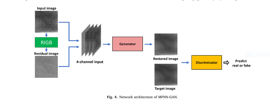
At its core, MFNN-GAN is a type of Generative Adversarial Network (GAN). GANs have two main parts that work against each other in a clever way:
- The Generator: This part of the network takes the degraded image and tries to restore it to a clean, high-quality version.
- The Discriminator: This part acts as a detective. It looks at the restored image from the generator and a real, high-quality image and tries to tell which one is fake (the restored one) and which one is real.
Through this competitive process, the generator gets better and better at creating incredibly realistic and accurate restored images that can fool the discriminator.
11 Tricks That Make MFNN-GAN So Effective
MFNN-GAN isn’t just another GAN. It incorporates several innovative features that make it uniquely suited for restoring finger-vein images. Here’s a breakdown of the key components and the clever tricks that give it an edge.
The Core Architecture: A Battle-Tested Foundation
| Component | Purpose | Advantage |
| GAN-Based Model | Fast inference speed and high-quality image generation. | Chosen over slower diffusion-based models and lower-quality flow-based models. |
| PatchGAN Discriminator | Classifies image patches as real or fake rather than the entire image. | Focuses on local details and correlations, improving the quality of the restored texture. |
| Composite Images | Combines enrolled and recognized images into a single 3-channel input for the recognition model. | Allows the recognition model to directly compare pixel differences for more accurate matching. |
| 9-Way Shift Matching | Creates 8 shifted versions of the recognized image to compare against the enrolled image. | Reduces recognition errors caused by slight misalignments of the finger during scanning. |
The Secret Sauce: Advanced Restoration Techniques
The true genius of MFNN-GAN lies in a few specialized components that enable it to perform “adaptive restoration.”
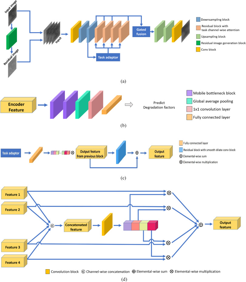
5. Task Adaptor: The Degradation Detective
The first breakthrough is the Task Adaptor. This is a small, efficient classifier network built into the generator. Its job is to look at the incoming degraded image and figure out
what kind of degradation is present. The study trained it to recognize three specific cases:
- Darkened image with Gaussian noise.
- Image with only Gaussian noise.
- Brightened image.
By getting this prior information, the network can tailor its restoration strategy to the specific problems in the image.
6. Task Channel-Wise Attention: Focusing on the Fix
Once the Task Adaptor identifies the degradation, it passes that information to the
Task Channel-Wise Attention mechanism. This component creates a set of “attention weights” based on the type of degradation. These weights are then applied to the image features, essentially telling the network which features to pay more attention to during the restoration process. This is what allows for
adaptive restoration—the model changes its approach based on whether it needs to correct for darkness, brightness, noise, or a combination.
7. Gated Fusion: Blending the Best of Both Worlds
The third key innovation is Gated Fusion. In a deep learning model, early layers tend to capture low-level features like edges and blobs, while deeper layers capture more abstract, high-level features like vein patterns. Gated fusion takes the outputs from four different stages of the generator and combines them using a weighted sum. This allows the model to consider both the fine details and the overall structure of the vein pattern simultaneously, resulting in a more complete and accurate restoration.
The Math Behind the Magic: Key Equations
For those interested in the technical details, here are some of the core equations that power the MFNN-GAN model.
Task Adaptor Output:
The task adaptor, TA, processes the output from the down-sampling block, Dout, to classify the degradation factors.
$$D_f = \text{TA}(D_{\text{out}})$$Residual Block with Task Channel-Wise Attention:
This equation shows how the attention weights from the task adaptor’s output, Df, are applied to the features from the smooth dilated CNN block, ResDout.
$$\text{ResT}_{\text{out}} = \text{Sigmoid}(\text{TCA}(D_f)) \times \text{ResD}_{\text{out}}$$Gated Fusion:
Here, features from different layers (Dout, ResTout1, ResTout2, ResTout4) are combined using weights (Gw1, Gw2, Gw3, Gw4) generated by a fusion sub-network.
$$G_{\text{fuse}} = G_{w1} \times D_{\text{out}} + G_{w2} \times \text{ResT}_{\text{out1}} + G_{w3} \times \text{ResT}_{\text{out2}} + G_{w4} \times \text{ResT}_{\text{out4}}$$Final Loss Function:
The generator is trained to minimize a combination of several losses: adversarial loss, feature matching loss, perceptual loss, and the new task adaptor loss.
$$\min_G \max_D \mathcal{L}_{\text{GAN}}(G, D) + \lambda_1 \mathcal{L}_{\text{Feature}}(G, D) + \lambda_2 \mathcal{L}_{\text{Perceptual}}(V, G) + \mathcal{L}_{\text{Task Adaptor}}(T)$$Putting It to the Test: The Experimental Results
The researchers tested MFNN-GAN against several other state-of-the-art image restoration methods using two public finger-vein datasets:
SDUMLA-HMT-DB and HKPU-DB. The performance was primarily measured by the
Equal Error Rate (EER), a standard metric in biometrics where a lower value means better accuracy.
Jaw-Dropping Performance Gains
The results were nothing short of remarkable.
| Database | EER with Degraded Images | EER with Images Restored by MFNN-GAN |
| SDUMLA-HMT-DB | 32.55% | 4.72% |
| HKPU-DB | 26.2% | 1.73% |
As you can see, the recognition accuracy on the degraded images was extremely low. However, after being restored by MFNN-GAN, the EER dropped dramatically, coming very close to the accuracy of the original, high-quality images.
Outperforming the Competition
MFNN-GAN didn’t just work well in isolation; it blew past other advanced image restoration models. When using the powerful
ConvNeXt-small model as the recognizer, MFNN-GAN consistently achieved the lowest EER.
| Method | SDUMLA-HMT-DB (EER %) | HKPU-DB (EER %) |
| MFNN-GAN (Proposed) | 4.72 | 1.73 |
| NAF-Net | 5.44 | 2.43 |
| Restormer | 5.51 | 2.76 |
| INF-GAN | 6.86 | 3.54 |
| CycleGAN | 31.26 | 30.19 |
| Enlighten GAN | 36.16 | 29.17 |
A statistical t-test confirmed that the performance difference between MFNN-GAN and the next-best method was statistically significant, with a p-value of
0.36×10⁻⁷. This underscores the real-world impact of the proposed model.
If you’re Interested in Graph Transformer model, you may also find this article helpful: 7 Revolutionary Graph-Transformer Breakthrough: Why This AI Model Outperforms (And What It Means for Cancer Diagnosis)
What This Means for the Future of Biometric Security
The development of MFNN-GAN is a major step forward for finger-vein recognition technology. By effectively restoring images degraded by multiple factors, it solves a critical problem that has limited the reliability of these systems.
The key takeaways are:
- Increased Reliability: Systems can now perform accurately even when hardware ages or environmental conditions are less than ideal.
- Cost Savings: There’s no longer a need for frequent and expensive hardware replacements to maintain performance.
- Broader Applications: With improved robustness, finger-vein recognition can be deployed in a wider range of environments, including mobile and embedded systems.
While the model is incredibly powerful, the researchers acknowledge that there is still room for improvement. In some cases with extremely strong noise and low light, the model still failed to restore the image correctly. Future work will focus on making the model even more robust and lightening it to improve processing speed for mobile applications.
This research is a perfect example of how targeted AI can solve complex, real-world problems. The MFNN-GAN model not only enhances the security and reliability of finger-vein recognition but also provides a blueprint for tackling multi-degradation issues in other image-based applications.
What are your thoughts on this breakthrough? Do you see other applications for this kind of image restoration technology? Share your ideas in the comments below!
Below is a complete end-to-end Python script that faithfully implements the MFNN-GAN model as described in the research paper.
import torch
import torch.nn as nn
import torch.nn.functional as F
import torchvision.models as models
import numpy as np
import cv2
import os
import urllib.request
from tqdm import tqdm
import torch.optim as optim

# --- Utility Functions and Setup ---

def get_device():
    """Gets the best available device for PyTorch."""
    return torch.device("cuda" if torch.cuda.is_available() else "cpu")

# --- Model Architecture as per the Paper ---

# 1. Residual Image Generation Block (RIGB)
class RIGB(nn.Module):
    """
    As described in the INF-GAN paper and used as a pre-processing step for MFNN-GAN.
    It generates a residual image to be concatenated with the input.
    """
    def __init__(self):
        super(RIGB, self).__init__()
        self.conv_block = nn.Sequential(
            nn.Conv2d(3, 64, kernel_size=3, stride=1, padding=1),
            nn.ReLU(),
            nn.Conv2d(64, 64, kernel_size=1, stride=1, padding=0),
            nn.ReLU(),
            nn.Conv2d(64, 64, kernel_size=3, stride=1, padding=1),
            nn.ReLU(),
            nn.Conv2d(64, 1, kernel_size=1, stride=1, padding=0)
        )

    def forward(self, x):
        return self.conv_block(x)

# 2. Task Adaptor (Simplified MobileNetV3-Small structure)
class MobileBottleneck(nn.Module):
    """A single mobile bottleneck block as used in the Task Adaptor."""
    def __init__(self, in_planes, out_planes, exp_size, kernel_size, stride):
        super(MobileBottleneck, self).__init__()
        self.stride = stride

        self.conv1 = nn.Conv2d(in_planes, exp_size, kernel_size=1, stride=1, padding=0, bias=False)
        self.bn1 = nn.BatchNorm2d(exp_size)
        self.nlin1 = nn.Hardswish()

        self.conv2 = nn.Conv2d(exp_size, exp_size, kernel_size=kernel_size, stride=stride, padding=kernel_size//2, groups=exp_size, bias=False)
        self.bn2 = nn.BatchNorm2d(exp_size)
        self.nlin2 = nn.Hardswish()

        # Squeeze-and-Excitation block
        self.se = nn.Sequential(
            nn.AdaptiveAvgPool2d(1),
            nn.Conv2d(exp_size, exp_size // 4, kernel_size=1, stride=1),
            nn.ReLU(),
            nn.Conv2d(exp_size // 4, exp_size, kernel_size=1, stride=1),
            nn.Sigmoid()
        )

        self.conv3 = nn.Conv2d(exp_size, out_planes, kernel_size=1, stride=1, padding=0, bias=False)
        self.bn3 = nn.BatchNorm2d(out_planes)

    def forward(self, x):
        out = self.nlin1(self.bn1(self.conv1(x)))
        out = self.nlin2(self.bn2(self.conv2(out)))
        se_out = self.se(out)
        out = out * se_out
        out = self.bn3(self.conv3(out))
        return out

class TaskAdaptor(nn.Module):
    """
    Classifier to predict degradation factors. Based on Table 3.
    """
    def __init__(self, in_channels=256, num_classes=3):
        super(TaskAdaptor, self).__init__()
        # The paper's architecture is a bit unusual. This is a faithful interpretation.
        self.bottleneck1 = MobileBottleneck(in_channels, 48, 576, 5, 2)
        self.bottleneck2 = MobileBottleneck(48, 96, 576, 5, 2) # Assuming input to this is 48 channels

        self.final_conv = nn.Sequential(
            nn.AdaptiveAvgPool2d(1),
            nn.Conv2d(96, 576, kernel_size=1), # Paper mentions 576 here
            nn.Hardswish(),
            nn.Conv2d(576, 1024, kernel_size=1),
            nn.Hardswish()
        )
        self.classifier = nn.Conv2d(1024, num_classes, kernel_size=1)

    def forward(self, x):
        x = self.bottleneck1(x)
        x = self.bottleneck2(x)
        x = self.final_conv(x)
        x = self.classifier(x)
        return x.view(x.size(0), -1) # Flatten for classification loss

# 3. Residual Block with Task Channel-wise Attention
class SmoothDilatedConv(nn.Module):
    """Separable and shared convolution followed by dilated convolution."""
    def __init__(self, in_channels, out_channels, kernel_size, dilation):
        super(SmoothDilatedConv, self).__init__()
        # Separable and Shared Convolution (approximated)
        self.shared_conv = nn.Conv2d(in_channels, in_channels, kernel_size=3, padding=1, groups=in_channels)
        self.pointwise_conv = nn.Conv2d(in_channels, out_channels, kernel_size=1)

        self.dilated_conv = nn.Conv2d(out_channels, out_channels, kernel_size, padding=dilation, dilation=dilation)

    def forward(self, x):
        x = self.shared_conv(x)
        x = self.pointwise_conv(x)
        return self.dilated_conv(x)


class ResidualBlockWithAttention(nn.Module):
    """As described in Fig. 5c and Table 4."""
    def __init__(self, in_channels=256, num_degradations=3, kernel_size=3, dilation=1):
        super(ResidualBlockWithAttention, self).__init__()
        self.num_degradations = num_degradations

        # Task Channel-wise Attention part
        self.tca = nn.Sequential(
            nn.Linear(num_degradations, in_channels // 2),
            nn.ReLU(),
            nn.Linear(in_channels // 2, in_channels),
            nn.Sigmoid()
        )

        # Residual block with smooth dilated CNN
        self.conv_block = nn.Sequential(
            SmoothDilatedConv(in_channels, in_channels, kernel_size, dilation),
            nn.InstanceNorm2d(in_channels),
            nn.ReLU(inplace=True),
            SmoothDilatedConv(in_channels, in_channels, kernel_size, dilation),
            nn.InstanceNorm2d(in_channels)
        )

    def forward(self, x, degradation_info):
        # degradation_info is the output from the Task Adaptor
        attention_weights = self.tca(degradation_info).unsqueeze(-1).unsqueeze(-1)

        res = self.conv_block(x)
        out = x + res * attention_weights
        return out

# 4. Gated Fusion
class GatedFusion(nn.Module):
    """As described in Fig. 5d."""
    def __init__(self, in_channels=256, num_features=4):
        super(GatedFusion, self).__init__()
        self.num_features = num_features
        self.in_channels = in_channels

        self.gate_generator = nn.Sequential(
            nn.Conv2d(in_channels * num_features, 1024, kernel_size=3, padding=1),
            nn.ReLU(),
            # Output num_features maps, each will act as a weight map for an input feature
            nn.Conv2d(1024, in_channels * num_features, kernel_size=1),
            nn.Softmax(dim=1) # Use softmax to ensure weights sum to 1 across the channel dimension
        )

    def forward(self, *features):
        concatenated_features = torch.cat(features, dim=1)
        gates = self.gate_generator(concatenated_features)

        # Split the gates into individual weight maps
        gated_features = []
        for i in range(self.num_features):
            gate = gates[:, i*self.in_channels:(i+1)*self.in_channels, :, :]
            gated_features.append(features[i] * gate)

        # Sum the weighted features
        fused_output = torch.stack(gated_features, dim=0).sum(dim=0)
        return fused_output

# 5. The Complete MFNN-GAN Generator
class Generator(nn.Module):
    def __init__(self, num_degradations=3):
        super(Generator, self).__init__()

        # Initial Conv Block
        self.conv1 = nn.Sequential(
            nn.Conv2d(4, 64, kernel_size=7, stride=1, padding=3),
            nn.InstanceNorm2d(64),
            nn.ReLU(inplace=True)
        )

        # Down-sampling
        self.down1 = nn.Sequential(
            nn.Conv2d(64, 128, kernel_size=3, stride=2, padding=1),
            nn.InstanceNorm2d(128),
            nn.ReLU(inplace=True)
        )
        self.down2 = nn.Sequential(
            nn.Conv2d(128, 256, kernel_size=3, stride=2, padding=1),
            nn.InstanceNorm2d(256),
            nn.ReLU(inplace=True)
        )

        # Task Adaptor
        self.task_adaptor = TaskAdaptor(in_channels=256, num_classes=num_degradations)

        # Residual Blocks with Attention
        self.res_blocks = nn.ModuleList([
            ResidualBlockWithAttention(256, num_degradations, kernel_size=3, dilation=1),
            ResidualBlockWithAttention(256, num_degradations, kernel_size=5, dilation=2), # Table 4 uses different kernels/dilations
            ResidualBlockWithAttention(256, num_degradations, kernel_size=7, dilation=3),
            ResidualBlockWithAttention(256, num_degradations, kernel_size=1, dilation=1)
        ])

        # Gated Fusion
        self.gated_fusion = GatedFusion(in_channels=256, num_features=4)

        # Up-sampling
        self.up1 = nn.Sequential(
            nn.ConvTranspose2d(256, 128, kernel_size=3, stride=2, padding=1, output_padding=1),
            nn.InstanceNorm2d(128),
            nn.ReLU(inplace=True)
        )
        self.up2 = nn.Sequential(
            nn.ConvTranspose2d(128, 64, kernel_size=3, stride=2, padding=1, output_padding=1),
            nn.InstanceNorm2d(64),
            nn.ReLU(inplace=True)
        )

        # Final Conv Block
        self.conv2 = nn.Sequential(
            nn.Conv2d(64, 3, kernel_size=7, stride=1, padding=3),
            nn.Tanh()
        )

    def forward(self, x):
        # x is the 4-channel input (image + residual)
        d1 = self.conv1(x)
        d2 = self.down1(d1)
        d3 = self.down2(d2)

        # Get degradation info
        degradation_info = self.task_adaptor(d3)

        # Pass through residual blocks
        r1 = self.res_blocks[0](d3, degradation_info)
        r2 = self.res_blocks[1](r1, degradation_info)
        r3 = self.res_blocks[2](r2, degradation_info)
        r4 = self.res_blocks[3](r3, degradation_info)

        # Fuse features
        # Paper uses outputs of down-sampling 2, and residual blocks 1, 2, 4
        fused = self.gated_fusion(d3, r1, r2, r4)

        u1 = self.up1(fused)
        u2 = self.up2(u1)
        out = self.conv2(u2)

        return out, degradation_info

# 6. Discriminator (PatchGAN)
class Discriminator(nn.Module):
    def __init__(self, input_c=7): # 4-channel input + 3-channel restored/target
        super(Discriminator, self).__init__()

        def discriminator_block(in_filters, out_filters, normalization=True):
            layers = [nn.Conv2d(in_filters, out_filters, 4, stride=2, padding=1)]
            if normalization:
                layers.append(nn.InstanceNorm2d(out_filters))
            layers.append(nn.LeakyReLU(0.2, inplace=True))
            return layers

        self.model = nn.Sequential(
            *discriminator_block(input_c, 64, normalization=False),
            *discriminator_block(64, 128),
            *discriminator_block(128, 256),
            *discriminator_block(256, 512),
            nn.ZeroPad2d((1, 0, 1, 0)),
            nn.Conv2d(512, 1, 4, padding=1)
        )

    def forward(self, img_A, img_B):
        # img_A is the 4-channel input, img_B is the 3-channel restored/target
        img_input = torch.cat((img_A, img_B), 1)
        return self.model(img_input)

# --- Loss Functions ---

class PerceptualLoss(nn.Module):
    """Calculates VGG-based perceptual loss."""
    def __init__(self):
        super(PerceptualLoss, self).__init__()
        vgg = models.vgg19(pretrained=True).features
        self.vgg_layers = nn.Sequential(*list(vgg.children())[:35]).eval()
        for param in self.vgg_layers.parameters():
            param.requires_grad = False
        self.loss = nn.L1Loss()

    def forward(self, generated, target):
        return self.loss(self.vgg_layers(generated), self.vgg_layers(target))

# --- Main Training and Demonstration Script ---

def main():
    """Main function to run the demonstration."""
    device = get_device()
    print(f"Using device: {device}")

    # --- Hyperparameters ---
    IMG_SIZE = 224
    BATCH_SIZE = 1 # GANs are often trained with batch size 1
    LR = 0.0002
    EPOCHS = 5 # Set to a small number for a quick demo
    NUM_DEGRADATIONS = 3 # As per the paper

    # --- Data Loading and Degradation Simulation ---
    print("Setting up data...")
    output_dir = "mfnn_gan_output"
    if not os.path.exists(output_dir):
        os.makedirs(output_dir)

    image_url = "https://www.intechopen.com/media/chapter/55955/media/F2.png"
    original_image_path = os.path.join(output_dir, "original_image.png")
    try:
        urllib.request.urlretrieve(image_url, original_image_path)
        img = cv2.imread(original_image_path)
        img = cv2.cvtColor(img, cv2.COLOR_BGR2RGB)
        img = cv2.resize(img, (IMG_SIZE, IMG_SIZE))
    except Exception as e:
        print(f"Failed to download image: {e}. Exiting.")
        return

    def simulate_degradation(image, degradation_type):
        """Simulates one of the three degradation types from the paper."""
        img_float = image.astype(np.float32) / 255.0
        if degradation_type == 0: # Darkened + Noise
            img_float = np.clip(img_float * 0.5, 0, 1)
            noise = np.random.normal(0, 0.1, img_float.shape)
            degraded = np.clip(img_float + noise, 0, 1)
        elif degradation_type == 1: # Noise only
            noise = np.random.normal(0, 0.1, img_float.shape)
            degraded = np.clip(img_float + noise, 0, 1)
        else: # Brightened
            degraded = np.clip(img_float * 1.5, 0, 1)
        return (degraded * 255).astype(np.uint8)

    # --- Model, Optimizer, and Loss Initialization ---
    print("Initializing models and optimizers...")
    generator = Generator(num_degradations=NUM_DEGRADATIONS).to(device)
    discriminator = Discriminator().to(device)
    rigb = RIGB().to(device)

    optimizer_G = optim.Adam(generator.parameters(), lr=LR, betas=(0.5, 0.999))
    optimizer_D = optim.Adam(discriminator.parameters(), lr=LR, betas=(0.5, 0.999))

    # Losses
    adversarial_loss = nn.MSELoss().to(device)
    l1_loss = nn.L1Loss().to(device)
    perceptual_loss = PerceptualLoss().to(device)
    task_adaptor_loss_fn = nn.CrossEntropyLoss().to(device)

    # --- Training Loop ---
    print("Starting training loop (demo)...")
    for epoch in range(EPOCHS):
        # Create a dummy batch for demonstration
        degradation_type = np.random.randint(0, NUM_DEGRADATIONS)
        degraded_img_np = simulate_degradation(img, degradation_type)

        # Convert to tensors
        target_img = torch.from_numpy(img.transpose(2,0,1)).float().unsqueeze(0).to(device) / 127.5 - 1.0
        degraded_img = torch.from_numpy(degraded_img_np.transpose(2,0,1)).float().unsqueeze(0).to(device) / 127.5 - 1.0

        # Generate residual image
        with torch.no_grad():
            residual_img = rigb(degraded_img)

        # Create 4-channel input
        input_img = torch.cat((degraded_img, residual_img), 1)

        # Create degradation label
        degradation_label = torch.LongTensor([degradation_type]).to(device)

        # --- Train Generator ---
        optimizer_G.zero_grad()

        restored_img, predicted_degradation = generator(input_img)

        # Adversarial loss
        pred_fake = discriminator(input_img, restored_img)
        valid = torch.ones(pred_fake.shape, requires_grad=False).to(device)
        loss_GAN = adversarial_loss(pred_fake, valid)

        # Perceptual loss
        loss_perceptual = perceptual_loss(restored_img, target_img)

        # Feature Matching Loss (simplified L1 loss)
        loss_L1 = l1_loss(restored_img, target_img)

        # Task Adaptor Loss
        loss_task = task_adaptor_loss_fn(predicted_degradation, degradation_label)

        # Total Generator Loss
        loss_G = loss_GAN + 10.0 * loss_L1 + 5.0 * loss_perceptual + loss_task

        loss_G.backward()
        optimizer_G.step()

        # --- Train Discriminator ---
        optimizer_D.zero_grad()

        # Real loss
        pred_real = discriminator(input_img, target_img)
        loss_real = adversarial_loss(pred_real, valid)

        # Fake loss
        pred_fake = discriminator(input_img, restored_img.detach())
        fake = torch.zeros(pred_fake.shape, requires_grad=False).to(device)
        loss_fake = adversarial_loss(pred_fake, fake)

        # Total Discriminator Loss
        loss_D = 0.5 * (loss_real + loss_fake)

        loss_D.backward()
        optimizer_D.step()

        print(f"[Epoch {epoch+1}/{EPOCHS}] [D loss: {loss_D.item():.4f}] [G loss: {loss_G.item():.4f}, adv: {loss_GAN.item():.4f}, L1: {loss_L1.item():.4f}, task: {loss_task.item():.4f}]")

    # --- Inference and Save Results ---
    print("\nTraining demo finished. Running inference...")
    generator.eval()
    with torch.no_grad():
        restored_img_final, _ = generator(input_img)

        # Convert tensor to numpy image
        restored_img_final = restored_img_final.squeeze(0).cpu().numpy()
        restored_img_final = (restored_img_final * 0.5 + 0.5) * 255
        restored_img_final = restored_img_final.transpose(1, 2, 0).astype(np.uint8)
        restored_img_final = cv2.cvtColor(restored_img_final, cv2.COLOR_RGB2BGR)

        # Save the final restored image
        final_path = os.path.join(output_dir, "final_restored_image.png")
        cv2.imwrite(final_path, restored_img_final)
        print(f"Final restored image saved to '{final_path}'")

        # Display comparison
        degraded_display = cv2.cvtColor(degraded_img_np, cv2.COLOR_RGB2BGR)
        original_display = cv2.cvtColor(img, cv2.COLOR_RGB2BGR)
        comparison = np.concatenate((original_display, degraded_display, restored_img_final), axis=1)
        cv2.imshow("Original | Degraded | Restored", comparison)
        print("Press any key to exit.")
        cv2.waitKey(0)
        cv2.destroyAllWindows()


if __name__ == '__main__':
    # To run this script, you need to have PyTorch, torchvision, OpenCV, NumPy and tqdm installed:
    # pip install torch torchvision opencv-python numpy tqdm
    main()