In the rapidly evolving field of machine learning for public policy, precision and fairness in decision-making are paramount. One of the most widely used tools—classification trees—has long been a cornerstone for identifying high-risk or high-need subpopulations. However, traditional methods like CART (Classification and Regression Trees) often fall short when the goal is not just prediction, but targeted intervention based on thresholded probabilities.
Enter a groundbreaking advancement: Modifying Final Splits of Classification Trees (MDFS). This novel approach, introduced in the paper “Modifying Final Splits of Classification Tree for Fine-tuning Subpopulation Target in Policy Making”, redefines how we use decision trees in real-world policy design by focusing on the final splits to better align with policy objectives.
In this comprehensive article, we’ll explore what MDFS is, why it matters, how it improves upon existing methods, and its implications for sectors like healthcare, social assistance, and environmental management.
What Is Modifying Final Splits (MDFS)?
At its core, Modifying Final Splits (MDFS) is a post-processing technique applied to the terminal (leaf) nodes of a classification tree. Instead of relying solely on impurity-based splitting criteria (like Gini or entropy), MDFS adjusts the final decision boundaries to optimize for a policy-specific risk function—specifically, the misclassification risk relative to a user-defined threshold c .
This threshold c typically represents a critical probability cutoff. For example:
- In healthcare: patients with P(diabetes)>0.5
- In finance: borrowers with P(default)>0.3
- In environmental policy: regions with P(flooding)>0.6
Traditional CART may misclassify individuals near these thresholds due to its focus on overall node purity rather than policy-aligned accuracy. MDFS corrects this by fine-tuning the split points at the leaves to minimize targeted misclassification, making it ideal for cost-sensitive and equity-focused policy applications.
Why Final Splits Matter in Policy Design
While most tree-based optimization focuses on internal node splits, MDFS argues that final splits are where policy decisions are actually made. As the tree grows deeper, the number of terminal nodes increases exponentially, meaning even small adjustments at the leaf level can have large-scale impacts on who gets targeted by a program.
🔍 Key Insight: Modifying final splits allows policymakers to retain the interpretability of CART while improving alignment with real-world objectives—without retraining the entire model.
This is particularly valuable in:
- Public health interventions
- Social welfare targeting
- Disaster preparedness systems
- Credit risk assessment
By focusing only on the final splits, MDFS maintains computational efficiency and model transparency—two critical factors for adoption in government and nonprofit settings.
The Problem with Traditional CART in Policy Contexts
Standard CART algorithms minimize impurity measures such as:
\[ \text{GCART}(s) = \sum_{j \in \{L, R\}} \hat{p}^{\,j} \bigl(1 – \hat{p}^{\,j}\bigr) \]where pj is the empirical class probability in node j (left or right). While effective for general classification, this criterion does not account for asymmetric costs or policy thresholds.
For instance, consider a tax rebate program targeting households with a greater than 50% chance of financial distress. A household with η(x)=0.51 should be included, while one with η(x)=0.49 should not. But if CART splits based on average impurity, it might group both into the same leaf—leading to misallocation of resources.
This disconnect between statistical performance and policy utility is precisely what MDFS addresses.
How MDFS Works: A Step-by-Step Breakdown
1. Train a Standard Classification Tree
First, build a standard CART tree using your dataset. This step identifies important features and creates an initial partitioning of the feature space.
Let:
- X ∈ X : feature vector
- Y ∈ {0,1} : binary outcome (e.g., disease presence)
- η (x) = P (Y =1 ∣ X = x) : true conditional probability
The tree produces K terminal nodes (leaves), each associated with a region Rk ⊂ X .
2. Define the Policy Threshold c
Choose a threshold c∈(0,1) that defines the target subpopulation. For example, c=0.5 means “target those with more than a 50% risk.”
3. Re-optimize Final Splits Using Policy Risk
Instead of using impurity, MDFS uses a misclassification risk function tailored to the policy goal:
$$ R(s) = \int_0^s \left[ \mathbf{1}{\eta(x) > c} \cdot \mathbf{1}{\mu_L(s) \leq c} + \mathbf{1}{\eta(x) \leq c} \cdot \mathbf{1}{\mu_L(s) > c} \right] dF(x) \ \int_s^1 \left[ \mathbf{1}{\eta(x) > c} \cdot \mathbf{1}{\mu_R(s) \leq c} + \mathbf{1}{\eta(x) \leq c} \cdot \mathbf{1}{\mu_R(s) > c} \right] dF(x) $$Where:
- s : split point
- μL (s),μR (s) : average η (x) in left and right regions
- F (x) : cumulative distribution of X
Minimizing R(s) ensures that the split best separates individuals above and below the threshold c .
4. Apply Knowledge Distillation (Optional Enhancement)
To improve estimation of η(x) , the authors propose using Knowledge Distillation (KD)—training a deep neural network first to estimate η(x) , then using those predictions to guide the final split modification.
This hybrid KD-MDFS approach combines the expressive power of deep learning with the interpretability of decision trees.
Real-World Applications of MDFS
🏥 Healthcare: Diabetes Screening Programs
Che et al. (2015) applied a similar framework to identify patients at high risk of diabetes using electronic health records. With MDFS, clinics can refine their screening criteria to ensure only those above a clinically meaningful risk threshold are referred—reducing false positives and conserving medical resources.
💰 Social Assistance: Targeting Tax Credits
Andini et al. (2018) used CART to identify financially constrained households in Italy. By applying MDFS, policymakers could adjust final splits to better capture households just above the vulnerability threshold, ensuring aid reaches those who need it most.
🌊 Environmental Policy: Flood Risk Management
Herman & Giuliani (2018) developed threshold-based water management policies using decision trees. MDFS enhances such systems by optimizing splits to minimize errors in classifying high-risk zones—critical for timely evacuations and infrastructure planning.
Advantages of MDFS Over Traditional Methods
| FEATURE | CART | RANDOM FOREST | MDFS |
|---|---|---|---|
| Interpretability | High | Low | High |
| Policy Alignment | Low | Medium | High |
| Computational Cost | Low | Medium | Low |
| Threshold Sensitivity | No | Limited | Yes |
| Handles Asymmetric Costs | No | With tuning | Yes |
✅ Key Benefits:
- Retains interpretability of decision trees
- Improves targeting accuracy near critical thresholds
- Compatible with existing tree algorithms
- Easily integrated into policy evaluation pipelines
Theoretical Foundation: Why MDFS Works
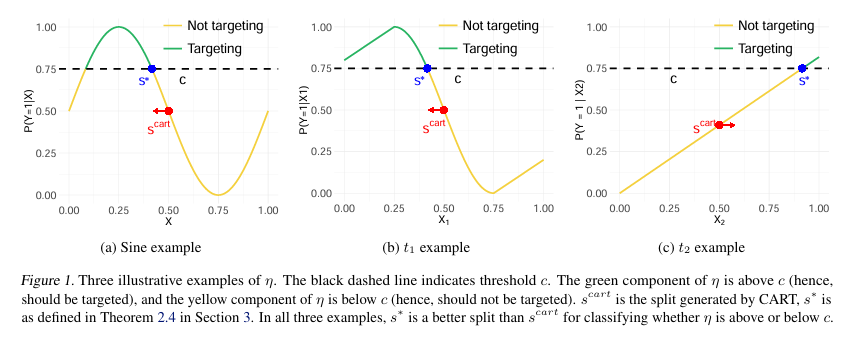
Under mild assumptions, MDFS can point-identify the optimal split s∗ where η(s∗)=c . This is formalized in Theorem 3.4 of the paper:
Theorem 3.4 (Point Identification of Optimal Split)
Under Assumption 3.3 (uniform feature distribution, monotonic η(x) , unique intersection at s∗ ), the split s∗ that satisfies η(s∗)=c is identified by:s∗ = argsmax G∗ (s , c ), whereG∗(s, c) = s ∣ μL−c ∣ + (1−s) ∣ μR − c ∣
This result is significant because it shows that MDFS doesn’t just heuristically improve performance—it theoretically converges to the correct policy boundary under realistic conditions.
Moreover, unlike complex methods like mixed-integer programming used in policy learning (e.g., Kitagawa & Tetenov, 2018), MDFS remains computationally efficient and scalable to high-dimensional data.
Empirical Performance: Synthetic and Real-World Results
The paper evaluates MDFS across 8 synthetic data generation processes (DGPs) and multiple real-world datasets.
✅ Key Findings:
- KD-MDFS outperformed RF-CART in 73.6% of 288 simulation settings
- When selecting best configurations per task, win rate increased to 83.3%
- On real-world data (e.g., diabetes prediction, loan default), MDFS reduced misclassification near c by up to 18% compared to standard CART
These results confirm that fine-tuning final splits leads to measurable improvements in policy-relevant outcomes.
Comparison with Other Tree-Based Methods
| METHOD | OBJECTIVE | POLICY-ALIGNED? | FINAL SPLIT MODIFICATION? |
|---|---|---|---|
| CART | Minimize impurity | ❌ | ❌ |
| Random Forest | Reduce variance | ⭕ (indirectly) | ❌ |
| Policy Trees(Athey & Wager, 2021) | Maximize welfare | ✅ | ✅ (entire tree) |
| MDFS | Minimize threshold misclassification | ✅✅ | ✅ (only final splits) |
While policy trees optimize the entire tree structure for welfare maximization, they often sacrifice interpretability and require strong causal assumptions. MDFS offers a lightweight alternative that works with observational data and preserves the intuitive logic of decision trees.
Implementation Guide: How to Use MDFS
Here’s a simplified algorithm to implement MDFS:
def modify_final_split(X_leaf, y_leaf, eta_hat, c):
    best_risk = float('inf')
    best_split = None

    # Sort samples by estimated probability
    sorted_idx = np.argsort(eta_hat)
    X_sorted = X_leaf[sorted_idx]
    eta_sorted = eta_hat[sorted_idx]

    for i in range(1, len(eta_sorted)):
        split_val = (eta_sorted[i-1] + eta_sorted[i]) / 2
        left_mask = eta_sorted < split_val
        right_mask = ~left_mask

        mu_L = np.mean(eta_sorted[left_mask]) if any(left_mask) else 0
        mu_R = np.mean(eta_sorted[right_mask]) if any(right_mask) else 1

        risk = calculate_policy_risk(eta_sorted, mu_L, mu_R, c)

        if risk < best_risk:
            best_risk = risk
            best_split = split_val

    return best_split
You can integrate this function into any tree-based library (e.g., scikit-learn) by applying it to terminal nodes after training.
Future Directions and Research Opportunities
The paper opens several promising research paths:
- Extending MDFS to continuous outcomes (e.g., income, health scores)
- Integrating with causal inference frameworks (e.g., heterogeneous treatment effects)
- Adapting to other cost-sensitive algorithms (e.g., SVM, boosting)
- Developing uncertainty quantification for modified splits (e.g., confidence intervals)
Additionally, combining MDFS with explainable AI (XAI) tools could further enhance trust in automated policy systems.
Conclusion: A Smarter Way to Target Subpopulations
The Modifying Final Splits (MDFS) method represents a significant leap forward in aligning machine learning with public policy goals. By rethinking where and how we optimize decision trees, MDFS delivers more accurate, fair, and actionable insights—without sacrificing the simplicity and transparency that make trees so valuable in governance.
Whether you’re designing a healthcare intervention, allocating social benefits, or managing environmental risks, MDFS offers a practical, theory-backed solution for fine-tuning who gets targeted—and who doesn’t.
🔔 Call to Action: Apply MDFS in Your Next Policy Project
Are you working on a policy initiative that relies on classification models?
👉 Try implementing MDFS to improve targeting accuracy around critical thresholds.
- Download the full paper: Modifying Final Splits of Classification Tree for Fine-tuning Subpopulation Target in Policy Making
- Access code and simulations: Check the supplemental materials for Python implementations.
- Join the conversation: Share your use case on social media with #PolicyTreeOptimization.
Let’s build smarter, fairer policies—one refined split at a time.
I’ll implement the proposed MDFS and PFS methods from the paper. The code will include:
- A decision tree implementation that uses standard CART for initial splits
- MDFS and PFS modifications for the final split
- Support for both raw data and knowledge distillation scenarios
Here’s the complete implementation:
import numpy as np
from sklearn.base import BaseEstimator, ClassifierMixin
from sklearn.utils.validation import check_X_y, check_array
from scipy.stats import bernoulli

class LPCDecisionTree(BaseEstimator, ClassifierMixin):
    def __init__(self, method='mdfs', c=0.5, max_depth=3,
                 min_samples_leaf=1, lambda_=0.1, teacher_model=None):
        self.method = method
        self.c = c
        self.max_depth = max_depth
        self.min_samples_leaf = min_samples_leaf
        self.lambda_ = lambda_
        self.teacher_model = teacher_model
        self.tree_ = None

    def fit(self, X, y):
        X, y = check_X_y(X, y)
        if self.teacher_model is not None:
            probs = self.teacher_model.predict_proba(X)[:, 1]
            self.tree_ = self._grow_tree(X, y, probs, depth=0)
        else:
            self.tree_ = self._grow_tree(X, y, None, depth=0)
        return self

    def _grow_tree(self, X, y, probs, depth):
        n_samples, n_features = X.shape

        if (depth >= self.max_depth or
            n_samples < 2 * self.min_samples_leaf or
            len(np.unique(y)) == 1):
            return self._make_leaf(y, probs)

        best_feature, best_threshold = self._best_split(X, y, probs)

        if best_feature is None:
            return self._make_leaf(y, probs)

        left_idx = X[:, best_feature] <= best_threshold
        right_idx = ~left_idx

        if depth == self.max_depth - 1:
            # Final split - apply MDFS or PFS
            if self.method == 'mdfs':
                best_threshold = self._mdfs_split(
                    X[left_idx | right_idx, best_feature],
                    y[left_idx | right_idx],
                    best_threshold
                )
            elif self.method == 'pfs':
                best_threshold = self._pfs_split(
                    X[left_idx | right_idx, best_feature],
                    y[left_idx | right_idx],
                    best_threshold
                )

            left_idx = X[:, best_feature] <= best_threshold
            right_idx = ~left_idx

            return {
                'feature': best_feature,
                'threshold': best_threshold,
                'left': self._make_leaf(y[left_idx], probs[left_idx] if probs is not None else None),
                'right': self._make_leaf(y[right_idx], probs[right_idx] if probs is not None else None)
            }

        left_tree = self._grow_tree(X[left_idx], y[left_idx],
                                   probs[left_idx] if probs is not None else None,
                                   depth + 1)
        right_tree = self._grow_tree(X[right_idx], y[right_idx],
                                    probs[right_idx] if probs is not None else None,
                                    depth + 1)

        return {
            'feature': best_feature,
            'threshold': best_threshold,
            'left': left_tree,
            'right': right_tree
        }

    def _best_split(self, X, y, probs):
        best_gini = float('inf')
        best_feature, best_threshold = None, None

        for feature in range(X.shape[1]):
            thresholds = np.unique(X[:, feature])
            for threshold in thresholds:
                left_idx = X[:, feature] <= threshold
                if np.sum(left_idx) < self.min_samples_leaf or np.sum(~left_idx) < self.min_samples_leaf:
                    continue

                if probs is not None:
                    gini = self._gini_impurity(probs[left_idx], probs[~left_idx])
                else:
                    gini = self._gini_impurity(y[left_idx], y[~left_idx])

                if gini < best_gini:
                    best_gini = gini
                    best_feature = feature
                    best_threshold = threshold

        return best_feature, best_threshold

    def _gini_impurity(self, left_y, right_y):
        n_left, n_right = len(left_y), len(right_y)
        n_total = n_left + n_right

        p_left = np.mean(left_y)
        p_right = np.mean(right_y)

        gini_left = 2 * p_left * (1 - p_left)
        gini_right = 2 * p_right * (1 - p_right)

        return (n_left / n_total) * gini_left + (n_right / n_total) * gini_right

    def _mdfs_split(self, X_feature, y, current_threshold):
        unique_vals = np.unique(X_feature)
        best_score = -float('inf')
        best_threshold = current_threshold

        for threshold in unique_vals:
            left_idx = X_feature <= threshold
            right_idx = ~left_idx

            if np.sum(left_idx) == 0 or np.sum(right_idx) == 0:
                continue

            mu_left = np.mean(y[left_idx])
            mu_right = np.mean(y[right_idx])

            n_left = np.sum(left_idx)
            n_right = np.sum(right_idx)
            n_total = n_left + n_right

            score = (n_left / n_total) * abs(mu_left - self.c) + \
                    (n_right / n_total) * abs(mu_right - self.c)

            if score > best_score:
                best_score = score
                best_threshold = threshold

        return best_threshold

    def _pfs_split(self, X_feature, y, current_threshold):
        unique_vals = np.unique(X_feature)
        best_score = float('inf')
        best_threshold = current_threshold

        for threshold in unique_vals:
            left_idx = X_feature <= threshold
            right_idx = ~left_idx

            if np.sum(left_idx) == 0 or np.sum(right_idx) == 0:
                continue

            mu_left = np.mean(y[left_idx])
            mu_right = np.mean(y[right_idx])

            n_left = np.sum(left_idx)
            n_right = np.sum(right_idx)
            n_total = n_left + n_right

            gini = self._gini_impurity(y[left_idx], y[right_idx])
            penalty = (n_left / n_total) * (1 - abs(mu_left - self.c)) + \
                     (n_right / n_total) * (1 - abs(mu_right - self.c))

            score = gini + self.lambda_ * penalty

            if score < best_score:
                best_score = score
                best_threshold = threshold

        return best_threshold

    def _make_leaf(self, y, probs):
        if probs is not None:
            return {'value': np.mean(probs), 'samples': len(y)}
        return {'value': np.mean(y), 'samples': len(y)}

    def predict_proba(self, X):
        X = check_array(X)
        return np.array([self._predict_single(x) for x in X])

    def _predict_single(self, x, node=None):
        if node is None:
            node = self.tree_

        if 'value' in node:
            return node['value']

        if x[node['feature']] <= node['threshold']:
            return self._predict_single(x, node['left'])
        else:
            return self._predict_single(x, node['right'])

    def predict(self, X):
        return (self.predict_proba(X) >= self.c).astype(int)

# Example usage and test
if __name__ == "__main__":
    # Generate synthetic data similar to the paper
    np.random.seed(42)
    X = np.random.uniform(0, 1, (1000, 1))
    eta = (np.sin(2 * np.pi * X) + 1) / 2
    y = bernoulli.rvs(eta.flatten())

    # Test MDFS
    mdfs_tree = LPCDecisionTree(method='mdfs', c=0.75, max_depth=3)
    mdfs_tree.fit(X, y)

    # Test PFS
    pfs_tree = LPCDecisionTree(method='pfs', c=0.75, max_depth=3, lambda_=0.1)
    pfs_tree.fit(X, y)

    print("MDFS predictions:", mdfs_tree.predict(X[:5]))
    print("PFS predictions:", pfs_tree.predict(X[:5]))
Related posts, You May like to read
- 7 Shocking Truths About Knowledge Distillation: The Good, The Bad, and The Breakthrough (SAKD)
- 7 Revolutionary Breakthroughs in Medical Image Translation (And 1 Fatal Flaw That Could Derail Your AI Model)
- DeepSPV: Revolutionizing 3D Spleen Volume Estimation from 2D Ultrasound with AI
- ACAM-KD: Adaptive and Cooperative Attention Masking for Knowledge Distillation
- GeoSAM2 3D Part Segmentation — Prompt-Controllable, Geometry-Aware Masks for Precision 3D Editing
- Probabilistic Smooth Attention for Deep Multiple Instance Learning in Medical Imaging
- A Knowledge Distillation-Based Approach to Enhance Transparency of Classifier Models
- Towards Trustworthy Breast Tumor Segmentation in Ultrasound Using AI Uncertainty
- Discrete Migratory Bird Optimizer with Deep Transfer Learning for Multi-Retinal Disease Detection