When Three Ultrasound Windows See What One Cannot:
MSFT-Net and the Sparse Fusion of Breast Tumor Intelligence
The Problem Nobody Wanted to Solve
Breast cancer is, in raw numbers, among the most frequently diagnosed cancers in women worldwide — roughly one in four newly detected female cancer cases. The mortality statistics are grimmer still. What is easy to miss in those figures, though, is how much of the diagnostic burden falls on a single radiologist sitting in a dark room, mentally juggling images from three different scanning technologies, each with its own noise profile, its own failure modes, and its own way of lying.
Conventional ultrasound — the grayscale B-mode scan that most people picture — gives you morphology. You see the shape of the lesion, its margins, whether its borders are smooth or spiky. What it cannot tell you is how stiff the tissue is, or whether abnormal blood vessels have been growing around the mass. For that, you need strain elastography (SE), which estimates tissue hardness by measuring deformation under probe pressure, and superb microvascular imaging (SMI), an advanced Doppler technique that pulls weak blood-flow signals from noisy backgrounds without the clutter of conventional color Doppler.
The problem runs deeper than just having three images to look at. Each modality is capturing a fundamentally different physical phenomenon. B-mode ultrasound records acoustic reflections. SMI tracks low-velocity hemodynamic pulsations over time — a temporal signal. SE measures the spatial stiffness gradient across tissue at a fixed plane — a spatial signal. Asking a single deep learning model to process all three modalities through a unified encoder is, the authors of this paper argue, like asking the same ear to simultaneously decode spoken language, music, and environmental noise — the signals interfere with each other before you ever learn anything useful.
The fundamental insight behind MSFT-Net is that not all cross-modal interactions are worth computing. Dense attention between modalities wastes capacity on noise-to-noise correlations. The architecture’s sparse mechanism learns to suppress precisely those interactions — keeping only what matters for malignancy prediction.
The team behind MSFT-Net — led by Jiahao Xu and Shuxin Zhuang from Shantou University and Sun Yat-sen University — took a different architectural approach. Rather than forcing all three modalities into a shared feature space and hoping the network would sort it out, they asked: what if we explicitly separate the temporal dynamics from the spatial structure first, then fuse only the most informative cross-modal interactions?
Three Modalities, Three Problems, Three Solutions
The MSFT-Net paper is organized around three specific challenges, and unusually for a medical imaging paper, each challenge maps directly to a dedicated architectural module. That structural clarity makes the paper easier to evaluate — you can test each solution in isolation, which the authors do with careful ablation experiments.
Problem 1: Heterogeneous Feature Distributions Across Modalities
SMI is fundamentally a temporal modality — the blood flow signals it captures evolve across frames as the probe scans through vascular structures. SE, by contrast, is best understood as a spatial modality — the stiffness gradient it visualizes is a property of tissue geometry at a given cross-section, not something that evolves meaningfully over the temporal sequence. Feeding both into the same encoder architecture — which is what most prior methods do — essentially asks the network to conflate these two very different kinds of information.
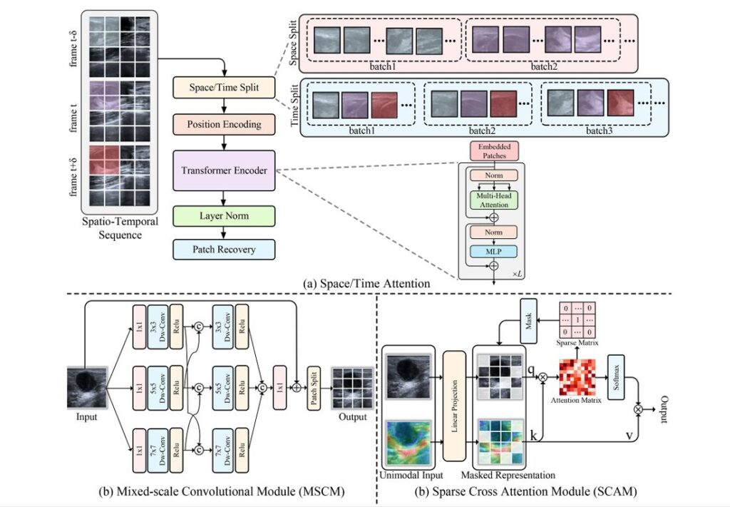
The Spatio-Temporal Decoupling Attention (STDA) architecture addresses this directly. Rather than using one encoder for both auxiliary modalities, STDA routes SMI through a temporal attention stream and SE through a spatial attention stream. The temporal attention, adapted from TimeSformer, ignores intra-frame pixel relationships and focuses entirely on how pixels at the same spatial position change across frames. The spatial attention does the opposite — it captures cross-pixel relationships within individual frames, independent of the sequence.
Positional encoding across both streams uses Fourier features rather than learnable position matrices:
The choice of Fourier encoding is worth noting. Learnable positional matrices add parameters and can overfit on limited medical datasets. Fourier features are fixed — they inject a broad frequency basis into the position representation, giving the model access to high-frequency spatial information without the weight cost. For a dataset of 458 patients, that kind of parameter efficiency matters.
The spatial attention computation for the SE stream captures inter-pixel relationships within each frame \( t \):
And the temporal attention for SMI attends to the same spatial position across different frames:
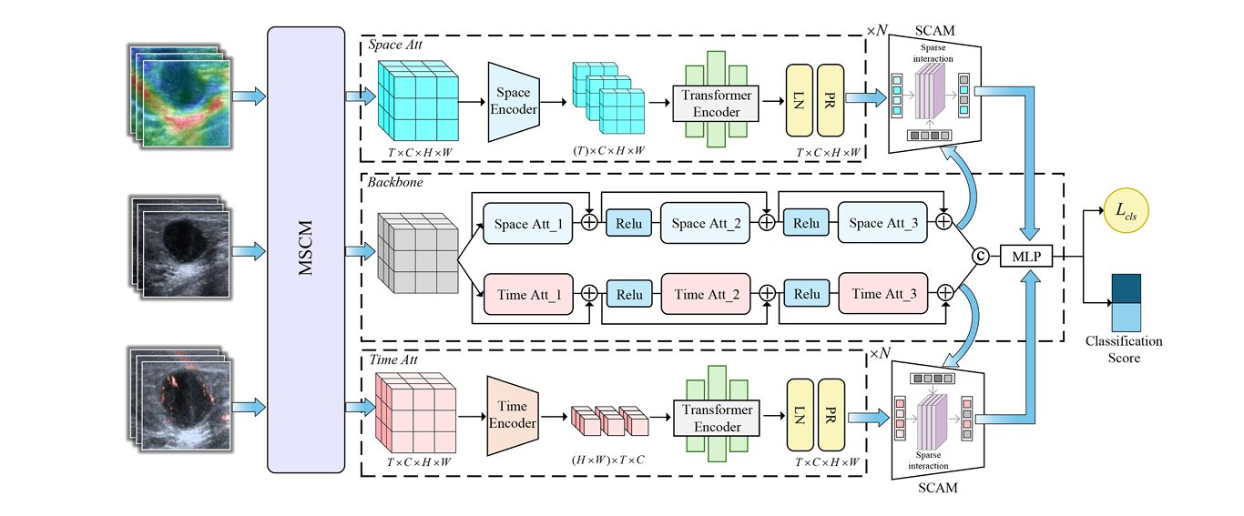
Problem 2: Single-Scale Feature Blindness
Here is something worth pausing on: a 3-centimeter malignant mass and a 5-millimeter early-stage lesion don’t just differ in size. They differ in the scale of features that distinguish them from benign tissue. Standard convolution with a fixed kernel size is, by definition, tuned for features at one spatial frequency. The tumor margins that matter for distinguishing invasive ductal carcinoma from a fibroadenoma look very different at 3×3 versus 7×7 pixel receptive fields.
The Mixed-Scale Convolution Module (MSCM) runs three parallel depth-wise convolution branches at 3×3, 5×5, and 7×7 kernels, then cross-connects them in a second stage before concatenation:
The cross-connections between branches in the second stage are what distinguishes MSCM from simple parallel multi-scale designs. A 3×3 branch informed by 5×5 features develops a receptive field that is neither purely local nor purely global — it sits at a scale that, in practice, aligns well with the textural irregularities in ultrasound tumor margins.
Problem 3: Redundant Cross-Modal Noise
That second problem is arguably the hardest. When you compute dense cross-attention between two multimodal feature sequences, you are computing similarity scores between every query token from one modality and every key token from the other. Most of those pairs carry no useful information — they correspond to acoustically shadowed regions in US matched against noise artifacts in SMI, or background tissue in SE matched against vessel signals that aren’t near the lesion.
The Sparse Cross-Attention Module (SCAM) replaces this dense operation with a learned sparse one. It computes the full attention matrix first, then applies top-k selection independently along both rows and columns:
The sparsity level is controlled by a learnable masking ratio \( w \in [0,1] \), with \( k = N – wN \). Through systematic search, the authors found optimal performance at \( w = 0.337 \) — meaning roughly two-thirds of cross-modal interactions survive masking. That is less than you might expect. It suggests that a substantial proportion of cross-modal attention, even in a well-designed system, is attending to things that don’t help classify tumors.
The Dataset: Why Collecting 458 Patients Is Harder Than It Sounds
There is no publicly available dataset of paired US, SMI, and SE breast tumor videos. The research team at Shantou Central Hospital had to build one from scratch — a clinical undertaking that required standardizing acquisition protocols across three scanning modes, coordinating radiologist annotations, and navigating patient privacy constraints.
The resulting dataset covers 458 patients: 196 malignant cases and 262 benign. The malignancy breakdown is clinically realistic — invasive carcinomas dominate (166 cases), with a smaller cohort of ductal carcinoma in situ (23 cases) and other malignant subtypes. The BI-RADS distribution skews toward the ambiguous middle categories (4a, 4b) where AI assistance has the most clinical value.
All videos were uniformly sampled to 16-frame sequences and center-cropped to 224×224 pixels. Importantly, the team excluded the additional B-mode images captured during SMI and SE scans — a subtle but important decision that prevents the model from learning easy shortcuts through incidentally duplicated US views.
“Performance disparities exist among individual modalities: ultrasound achieves superior classification accuracy due to its simultaneous capture of dynamic tumor characteristics and static morphological information.” — Xu, Zhuang et al., Medical Image Analysis, 2026
What the Numbers Actually Show
Five-fold cross-validation results are reported across six metrics. The headline accuracy of 92.55% is strong, but the more clinically meaningful number is the AUC of 98.94% — that describes global discriminability between malignant and benign cases across all operating thresholds, which is what actually matters when a radiologist is calibrating their decision sensitivity.
| Method | Type | ACC (%) | SEN (%) | SPE (%) | AUC (%) | F1 (%) |
|---|---|---|---|---|---|---|
| X3D | 3D CNN | 71.43 | 81.25 | 64.95 | 83.51 | 69.33 |
| I3D | 3D CNN | 73.29 | 85.94 | 64.95 | 87.05 | 71.90 |
| C3D | 3D CNN | 76.40 | 76.56 | 76.29 | 88.66 | 72.06 |
| Video-Swin | Transformer | 73.29 | 84.38 | 65.98 | 86.11 | 71.52 |
| VidTr | Transformer | 75.16 | 84.38 | 69.07 | 86.20 | 72.97 |
| AdaMAE | Masked AE | 77.64 | 82.81 | 74.23 | 90.32 | 74.65 |
| TransMed | Multimodal | 80.09 | 76.46 | 81.95 | 92.97 | 75.14 |
| TimeSformer | Transformer | 81.37 | 76.56 | 84.54 | 92.45 | 76.56 |
| MSFT-Net | Proposed | 92.55 | 90.62 | 93.81 | 98.94 | 90.62 |
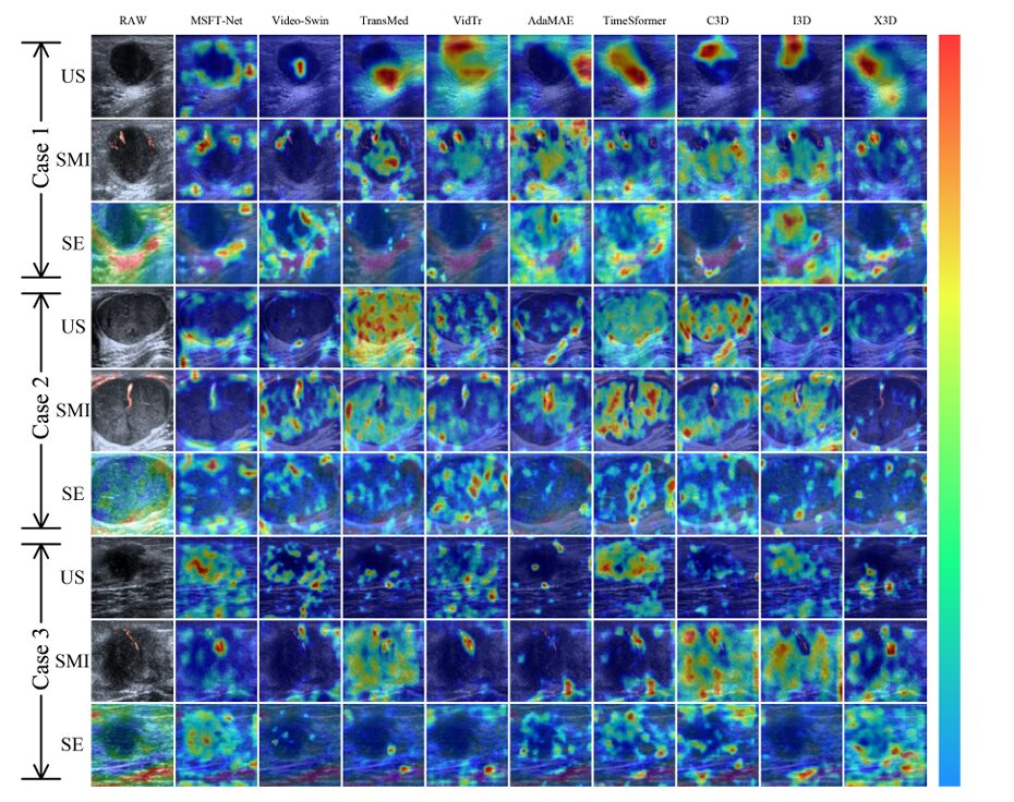
The 3D convolutional networks cluster between 71–76% accuracy, which gives you a sense of how much the transformer-based architectures actually add. But the more interesting comparison is between TimeSformer — the direct predecessor to MSFT-Net’s backbone — and the full model. MSFT-Net gains more than 11 percentage points in accuracy over TimeSformer, with a sensitivity jump from 76.56% to 90.62%. That sensitivity improvement matters most clinically: missing a malignant case is the failure mode that costs lives.
The ablation results are equally instructive. Add STDA alone: +5 percentage points over backbone. Add MSCM alone: +1.2 points. Add SCAM alone: +3.1 points. Add all three together: +9.9 points — more than the sum of the parts. That non-linearity in the ablation is the architectural fingerprint of a well-designed system: each module creates feature representations that the other modules can exploit more effectively.
Generalization to Brain Tumors: An Honest Validation
One of the more credible aspects of this paper is the decision to test MSFT-Net on the publicly available BraTS’21 brain tumor MRI dataset — a completely different disease, different imaging modality (MRI vs. ultrasound), and different classification task. On the BraTS’21 MGMT methylation classification task, MSFT-Net achieves 94.23% accuracy, outperforming the prior best reported result of 93.69% from LCDEiT.
That generalization doesn’t happen by accident. What transfers between the two domains is the structural logic of MSFT-Net’s design: heterogeneous modalities (T1, T1Gd, T2 in BraTS’21; US, SMI, SE in the breast dataset) benefit from decoupled spatial and temporal processing, and multi-scale feature extraction handles both the macro structures of glioblastoma and the micro-textural patterns of breast masses. The sparse attention mechanism proves equally effective at filtering cross-modal noise in MRI sequences as in ultrasound videos.
MSFT-Net’s performance on BraTS’21 — a dataset it was never designed for — is the strongest evidence that its core design decisions solve a general problem in multimodal medical imaging, not just the specific quirks of the breast tumor dataset. That breadth of applicability is rare in architectures this specialized.
What This Architecture Still Gets Wrong
None of this should paper over the limitations. The breast tumor video dataset of 458 patients is still small by the standards of deep learning in medical imaging. Five-fold cross-validation is methodologically sound, but standard deviations on key metrics are notable — accuracy variance of ±2.11 percentage points means that on an unlucky fold split, MSFT-Net might not clearly outperform a strong TimeSformer baseline.
The modality acquisition protocol is also demanding. Getting all three modalities — B-mode US, SMI, and SE — in the same clinical session requires specific equipment (the Canon Aplio i800 system was used here), trained operators, and careful standardization. In many clinical settings globally, SE and SMI are not routine. A system that requires three specialized scans to function is not yet a tool you can deploy in a community radiology center in rural China or rural anywhere.
There is also the matter of the optimal masking ratio. The paper reports \( w = 0.337 \) as the empirically derived optimum for this dataset. Whether that value generalizes to other tissue types, imaging equipment, or patient populations is an open question. A learnable masking ratio helps, but the sensitivity curve in Figure 9 of the paper shows performance collapsing quickly above \( w = 0.5 \) — the system has real tolerance limits.
Conclusion: The Intelligence Is in the Sparsity
There is a quiet insight buried in the SCAM results that deserves to be named directly. The fact that masking roughly a third of cross-modal interactions actually improves performance — rather than hurting it — tells you something important about how multimodal medical imaging systems fail. They don’t usually fail because they lack information. They fail because they attend to the wrong information, drowning the signal in noise. MSFT-Net’s contribution is partly about what it adds — the STDA decoupling, the multi-scale convolutions — and partly about what it deliberately removes.
That philosophy — selective attention as an act of discipline, not just efficiency — resonates well beyond breast tumor classification. The modality heterogeneity problem that STDA addresses is present wherever different imaging technologies are combined: PET/CT fusion, multiparametric MRI in prostate cancer, combined fluorescence and structural imaging in surgical guidance. The architectural template that works for US+SMI+SE video should transfer readily to those domains, with appropriate substitution of the decoupling strategy to match each modality’s dominant physical information axis.
The clinical story is also compelling. A system achieving 90.62% sensitivity with 93.81% specificity on an independent test set — where the ground truth comes from biopsy — is meaningfully better than reported inter-observer agreement rates between radiologists on ambiguous BI-RADS category 4 lesions. That doesn’t make it ready for deployment, but it puts it squarely in the category of methods worth rigorous prospective clinical evaluation.
The path from here to clinical deployment is not short, and the authors know it. Real-time inference, regulatory clearance, integration with existing PACS workflows, prospective validation on diverse patient populations — each step represents years of work. But the architectural problem that stopped previous systems from using all three modalities effectively has been genuinely addressed. That is the durable contribution, independent of the accuracy numbers on any particular dataset.
In multimodal medical imaging, the hard question has never been “can we acquire more data?” We can almost always acquire more data. The hard question is: “do we know which data, from which modality, at which moment, actually changes what we should think about this patient?” MSFT-Net makes a credible attempt to answer that question architecturally. That alone makes it worth understanding.
Complete Proposed Model Code (PyTorch)
The implementation below covers the full MSFT-Net architecture as described in the paper — MSCM, STDA (spatial + temporal attention streams), SCAM with learned sparse masking, the combined loss, and a smoke test matching the paper’s experimental configuration. Each module maps directly to a numbered section in the methodology.
# ============================================================
# MSFT-Net: Multimodal Sparse Fusion Transformer Network
# for Breast Tumor Classification
# Reference: Xu et al., Medical Image Analysis, Vol.110, 2026
# DOI: 10.1016/j.media.2026.103966
# GitHub: https://github.com/XuuuuJH-OvO/MSFT-Net
# ============================================================

import torch
import torch.nn as nn
import torch.nn.functional as F
import math


# ────────────────────────────────────────────────────────────
# 1. FOURIER POSITIONAL ENCODING
# ────────────────────────────────────────────────────────────
class FourierPositionalEncoding(nn.Module):
    """
    Fixed sinusoidal Fourier positional encoding.
    Reduces model parameters vs. learnable position matrices
    while preserving high-frequency spatial information.
    (Eq. 2 in paper)
    """
    def __init__(self, d_model: int, max_len: int = 512, f0: float = 10000.0):
        super().__init__()
        self.d_model = d_model
        pe = torch.zeros(max_len, d_model)
        position = torch.arange(0, max_len).unsqueeze(1).float()
        div_term = f0 ** (torch.arange(0, d_model, 2).float() / d_model)
        pe[:, 0::2] = torch.sin(position / div_term)
        pe[:, 1::2] = torch.cos(position / div_term)
        self.register_buffer('pe', pe.unsqueeze(0))

    def forward(self, x):
        # x: (B, seq_len, d_model)
        return x + self.pe[:, :x.size(1)]


# ────────────────────────────────────────────────────────────
# 2. MIXED-SCALE CONVOLUTION MODULE (MSCM)
# ────────────────────────────────────────────────────────────
class MSCM(nn.Module):
    """
    Mixed-Scale Convolution Module.
    Replaces standard convolutional projection with three
    parallel depth-wise conv branches (3x3, 5x5, 7x7),
    cross-connected in a second stage for multi-scale fusion.
    (Eq. 8 in paper)
    """
    def __init__(self, in_channels: int, hidden_dim: int = 36,
                 out_channels: int = 32, patch_size: int = 16):
        super().__init__()
        # Channel expansion
        self.expand = nn.Sequential(
            nn.Conv2d(in_channels, out_channels, 1),
            nn.LayerNorm([out_channels, 1, 1])  # applied after expand
        )
        # First stage: 3 parallel DW-Conv branches
        self.dwc3_1  = self._dwc(out_channels, 3, hidden_dim)
        self.dwc5_1  = self._dwc(out_channels, 5, hidden_dim)
        self.dwc7_1  = self._dwc(out_channels, 7, hidden_dim)
        # Second stage: cross-connected branches
        self.dwc3_2  = self._dwc(hidden_dim * 2, 3, hidden_dim)
        self.dwc5_2  = self._dwc(hidden_dim * 2, 5, hidden_dim)
        self.dwc7_2  = self._dwc(hidden_dim * 2, 7, hidden_dim)
        # Output projection to patch embedding dimension
        self.proj = nn.Conv2d(hidden_dim * 3, out_channels,
                              kernel_size=patch_size, stride=patch_size)
        self.relu = nn.ReLU(inplace=True)

    def _dwc(self, c_in, k, c_out):
        pad = k // 2
        return nn.Sequential(
            nn.Conv2d(c_in, c_in, k, padding=pad, groups=c_in, bias=False),
            nn.Conv2d(c_in, c_out, 1, bias=False),
            nn.ReLU(inplace=True)
        )

    def forward(self, x):
        # x: (B, C, H, W)
        B, C, H, W = x.shape
        h = self.expand[0](x)
        h = self.relu(h)
        # Stage 1
        z1 = self.dwc3_1(h)
        s1 = self.dwc5_1(h)
        p1 = self.dwc7_1(h)
        # Stage 2 — cross connections
        z2 = self.dwc3_2(torch.cat([z1, s1], dim=1))
        s2 = self.dwc5_2(torch.cat([s1, p1], dim=1))
        p2 = self.dwc7_2(torch.cat([z1, p1], dim=1))
        # Concat and project to patch embeddings
        out = self.proj(torch.cat([z2, s2, p2], dim=1))
        return out  # (B, embed_dim, H/patch, W/patch)


# ────────────────────────────────────────────────────────────
# 3. SPARSE CROSS-ATTENTION MODULE (SCAM)
# ────────────────────────────────────────────────────────────
class SCAM(nn.Module):
    """
    Sparse Cross-Attention Module.
    Computes cross-modal attention, then applies top-k masking
    independently on both rows AND columns of the attention matrix.
    Controlled by learnable masking ratio w ∈ [0,1].
    (Eq. 9–13 in paper)
    """
    def __init__(self, d_model: int = 768, n_heads: int = 8,
                 init_mask_ratio: float = 0.25, dropout: float = 0.5):
        super().__init__()
        self.d_model = d_model
        self.n_heads = n_heads
        self.head_dim = d_model // n_heads
        self.scale = self.head_dim ** -0.5
        # Learnable masking ratio
        self.mask_ratio = nn.Parameter(torch.tensor(init_mask_ratio))
        # Linear projections for two-layer SCAM
        self.fq1 = nn.Linear(d_model, d_model)
        self.fk1 = nn.Linear(d_model, d_model)
        self.fv1 = nn.Linear(d_model, d_model)
        self.fq2 = nn.Linear(d_model, d_model)
        self.fk2 = nn.Linear(d_model, d_model)
        self.fv2 = nn.Linear(d_model, d_model)
        self.out_proj = nn.Linear(d_model, d_model)
        self.dropout = nn.Dropout(dropout)
        self.norm = nn.LayerNorm(d_model)

    def _sparse_attn(self, Q, K, V, w):
        """
        Core sparse attention: compute full attention scores,
        mask bottom-(1-k) interactions to -inf, apply softmax.
        Row-wise AND column-wise top-k selection.
        """
        B, H, N, D = Q.shape
        alpha = torch.matmul(Q, K.transpose(-2, -1)) * self.scale  # (B,H,N,N)
        k = max(1, int(N * (1.0 - w.clamp(0, 0.99).item())))
        # Row-wise top-k thresholds
        t_row, _ = torch.topk(alpha, k, dim=-1)
        thresh_row = t_row[..., -1].unsqueeze(-1)
        # Column-wise top-k thresholds
        t_col, _ = torch.topk(alpha, k, dim=-2)
        thresh_col = t_col[..., -1, :].unsqueeze(-2)
        # Mask: keep only if passes BOTH row and column threshold
        mask = (alpha >= thresh_row) & (alpha >= thresh_col)
        alpha = alpha.masked_fill(~mask, float('-inf'))
        attn = F.softmax(alpha, dim=-1)
        attn = self.dropout(attn)
        return torch.matmul(attn, V)

    def _reshape_heads(self, x):
        B, N, D = x.shape
        return x.reshape(B, N, self.n_heads, self.head_dim).transpose(1, 2)

    def forward(self, z1, z2):
        """
        z1, z2: (B, N, d_model) — features from two modalities
        Returns fused feature (B, N, d_model)
        """
        w = self.mask_ratio
        B, N, _ = z1.shape
        # Layer 1: z1 as query, z2 as key/value
        Q1 = self._reshape_heads(self.fq1(z1))
        K1 = self._reshape_heads(self.fk1(z2))
        V1 = self._reshape_heads(self.fv1(z2))
        f1 = self._sparse_attn(Q1, K1, V1, w)
        f1 = f1.transpose(1, 2).reshape(B, N, self.d_model)
        f1 = self.norm(f1)
        # Layer 2: z2 as query, f1 as key/value (hierarchical design)
        Q2 = self._reshape_heads(self.fq2(z2))
        K2 = self._reshape_heads(self.fk2(f1))
        V2 = self._reshape_heads(self.fv2(f1))
        f2 = self._sparse_attn(Q2, K2, V2, w)
        f2 = f2.transpose(1, 2).reshape(B, N, self.d_model)
        return self.out_proj(f2)


# ────────────────────────────────────────────────────────────
# 4. SPATIO-TEMPORAL DECOUPLING ATTENTION (STDA)
# ────────────────────────────────────────────────────────────
class SpatialAttentionBlock(nn.Module):
    """
    Single spatial attention block for SE features.
    Computes self-attention across spatial positions within each frame,
    preserving temporal independence. (Eq. 3–5 in paper)
    """
    def __init__(self, d_model: int, n_heads: int, mlp_ratio: int = 4,
                 dropout: float = 0.5):
        super().__init__()
        self.norm1 = nn.LayerNorm(d_model, eps=1e-6)
        self.norm2 = nn.LayerNorm(d_model, eps=1e-6)
        self.attn = nn.MultiheadAttention(d_model, n_heads,
                                          dropout=dropout, batch_first=True)
        self.mlp = nn.Sequential(
            nn.Linear(d_model, d_model * mlp_ratio),
            nn.GELU(),
            nn.Dropout(dropout),
            nn.Linear(d_model * mlp_ratio, d_model),
            nn.Dropout(dropout)
        )

    def forward(self, x, T: int):
        """
        x: (B*T, N_spatial+1, d_model) — process each frame independently
        T: number of frames
        """
        res = x
        x = self.norm1(x)
        x, _ = self.attn(x, x, x)
        x = x + res
        x = x + self.mlp(self.norm2(x))
        return x


class TemporalAttentionBlock(nn.Module):
    """
    Single temporal attention block for SMI features.
    Attends across frames at the same spatial position,
    capturing hemodynamic evolution. (Eq. 6–7 in paper)
    """
    def __init__(self, d_model: int, n_heads: int, mlp_ratio: int = 4,
                 dropout: float = 0.5):
        super().__init__()
        self.norm1 = nn.LayerNorm(d_model, eps=1e-6)
        self.norm2 = nn.LayerNorm(d_model, eps=1e-6)
        self.attn = nn.MultiheadAttention(d_model, n_heads,
                                          dropout=dropout, batch_first=True)
        self.mlp = nn.Sequential(
            nn.Linear(d_model, d_model * mlp_ratio),
            nn.GELU(),
            nn.Dropout(dropout),
            nn.Linear(d_model * mlp_ratio, d_model),
            nn.Dropout(dropout)
        )

    def forward(self, x, N: int):
        """
        x: (B*N_spatial, T, d_model) — process each spatial position over time
        N: number of spatial patches
        """
        res = x
        x = self.norm1(x)
        x, _ = self.attn(x, x, x)
        x = x + res
        x = x + self.mlp(self.norm2(x))
        return x


class STDAEncoder(nn.Module):
    """
    Spatio-Temporal Decoupling Attention encoder.
    Routes SE videos through spatial attention layers;
    routes SMI videos through temporal attention layers.
    (Section 3.1 in paper — depth: SE=6 layers, SMI=5 layers)
    """
    def __init__(self, d_model: int = 768, n_heads: int = 8,
                 spatial_depth: int = 6, temporal_depth: int = 5,
                 mlp_ratio: int = 4, dropout: float = 0.5):
        super().__init__()
        self.spatial_layers = nn.ModuleList([
            SpatialAttentionBlock(d_model, n_heads, mlp_ratio, dropout)
            for _ in range(spatial_depth)
        ])
        self.temporal_layers = nn.ModuleList([
            TemporalAttentionBlock(d_model, n_heads, mlp_ratio, dropout)
            for _ in range(temporal_depth)
        ])
        self.norm_space = nn.LayerNorm(d_model)
        self.norm_time  = nn.LayerNorm(d_model)

    def encode_spatial(self, x_se):
        """SE stream: spatial attention per frame. x_se: (B,T,N+1,D)"""
        B, T, N1, D = x_se.shape
        x = x_se.reshape(B * T, N1, D)
        for layer in self.spatial_layers:
            x = layer(x, T)
        x = self.norm_space(x)
        return x.reshape(B, T, N1, D)[:, :, 0]  # CLS token per frame → (B,T,D)

    def encode_temporal(self, x_smi):
        """SMI stream: temporal attention per spatial patch. x_smi: (B,T,N+1,D)"""
        B, T, N1, D = x_smi.shape
        x = x_smi.permute(0, 2, 1, 3).reshape(B * N1, T, D)
        for layer in self.temporal_layers:
            x = layer(x, N1)
        x = self.norm_time(x)
        return x.reshape(B, N1, T, D).mean(dim=2)  # temporal mean pool → (B,N+1,D)

    def forward(self, x_se, x_smi):
        space_feat = self.encode_spatial(x_se)   # (B, T, D)
        time_feat  = self.encode_temporal(x_smi)  # (B, N+1, D)
        return space_feat, time_feat


# ────────────────────────────────────────────────────────────
# 5. US BACKBONE (simplified TimeSformer-style)
# ────────────────────────────────────────────────────────────
class USBackbone(nn.Module):
    """
    US classification backbone: dual-stream TimeSformer-style
    with 6 spatial + 6 temporal attention layers, d_model=768.
    """
    def __init__(self, d_model: int = 768, n_heads: int = 12, depth: int = 6,
                 dropout: float = 0.5):
        super().__init__()
        self.spatial_layers = nn.ModuleList([
            SpatialAttentionBlock(d_model, n_heads, dropout=dropout) for _ in range(depth)
        ])
        self.temporal_layers = nn.ModuleList([
            TemporalAttentionBlock(d_model, n_heads, dropout=dropout) for _ in range(depth)
        ])
        self.norm = nn.LayerNorm(d_model)

    def forward(self, x):
        # x: (B, T, N+1, D)
        B, T, N1, D = x.shape
        # Alternate spatial/temporal attention layers
        for sp, tm in zip(self.spatial_layers, self.temporal_layers):
            x_sp = sp(x.reshape(B * T, N1, D), T).reshape(B, T, N1, D)
            x_tm = tm(x.permute(0, 2, 1, 3).reshape(B * N1, T, D), N1)
            x_tm = x_tm.reshape(B, N1, T, D).permute(0, 2, 1, 3)
            x = x_sp + x_tm + x  # residual
        x = self.norm(x)
        return x[:, 0, 0]  # global CLS token → (B, D)


# ────────────────────────────────────────────────────────────
# 6. PATCH EMBEDDING HELPER
# ────────────────────────────────────────────────────────────
class VideoEmbedding(nn.Module):
    """Convert video clips to patch token sequences using MSCM."""
    def __init__(self, img_size: int = 224, patch_size: int = 16,
                 in_channels: int = 3, d_model: int = 768):
        super().__init__()
        self.n_patches = (img_size // patch_size) ** 2
        self.mscm = MSCM(in_channels, out_channels=d_model, patch_size=patch_size)
        self.cls_token = nn.Parameter(torch.zeros(1, 1, d_model))
        self.pos_enc = FourierPositionalEncoding(d_model, self.n_patches + 1)
        nn.init.trunc_normal_(self.cls_token, std=0.02)

    def forward(self, video):
        """video: (B, T, C, H, W) → (B, T, N+1, d_model)"""
        B, T, C, H, W = video.shape
        frames = video.reshape(B * T, C, H, W)
        patches = self.mscm(frames)              # (B*T, D, h, w)
        D = patches.shape[1]
        tokens = patches.flatten(2).transpose(1, 2)  # (B*T, N, D)
        cls = self.cls_token.expand(B * T, -1, -1)
        tokens = torch.cat([cls, tokens], dim=1)  # (B*T, N+1, D)
        tokens = self.pos_enc(tokens)
        return tokens.reshape(B, T, tokens.shape[1], D)


# ────────────────────────────────────────────────────────────
# 7. FULL MSFT-Net MODEL
# ────────────────────────────────────────────────────────────
class MSFTNet(nn.Module):
    """
    Multimodal Sparse Fusion Transformer Network (MSFT-Net).

    Inputs: trimodal video clips (US, SMI, SE)
    Output: binary classification logits (benign=0, malignant=1)

    Architecture:
      1. MSCM patch embedding for each modality
      2. US → dual-stream TimeSformer backbone
      3. SE → STDA spatial encoder (6 layers)
      4. SMI → STDA temporal encoder (5 layers)
      5. SCAM sparse cross-attention fusion (SE↔SMI)
      6. Feature concatenation + MLP classifier
    """
    def __init__(self,
                 img_size: int = 224,
                 patch_size: int = 16,
                 n_frames: int = 16,
                 d_model: int = 768,
                 n_heads_backbone: int = 12,
                 n_heads_stda: int = 8,
                 backbone_depth: int = 6,
                 spatial_depth: int = 6,
                 temporal_depth: int = 5,
                 n_classes: int = 2,
                 dropout: float = 0.5):
        super().__init__()
        self.d_model = d_model

        # Patch embedding (shared MSCM per modality)
        self.embed_us  = VideoEmbedding(img_size, patch_size, 3, d_model)
        self.embed_smi = VideoEmbedding(img_size, patch_size, 3, d_model)
        self.embed_se  = VideoEmbedding(img_size, patch_size, 3, d_model)

        # US backbone
        self.backbone = USBackbone(d_model, n_heads_backbone, backbone_depth, dropout)

        # STDA for SMI (temporal) and SE (spatial)
        self.stda = STDAEncoder(d_model, n_heads_stda,
                                spatial_depth, temporal_depth, dropout=dropout)

        # SCAM: fuse temporal (SMI) and spatial (SE) features
        self.scam = SCAM(d_model, n_heads_stda, dropout=dropout)

        # Feature fusion MLP (US_cls + SCAM_fused_cls)
        self.fusion_mlp = nn.Sequential(
            nn.Linear(d_model * 2, d_model),
            nn.GELU(),
            nn.Dropout(dropout),
            nn.Linear(d_model, d_model)
        )

        # Classification head
        self.classifier = nn.Sequential(
            nn.LayerNorm(d_model),
            nn.Linear(d_model, n_classes)
        )

        self._init_weights()

    def _init_weights(self):
        for m in self.modules():
            if isinstance(m, nn.Linear):
                nn.init.trunc_normal_(m.weight, std=0.02)
                if m.bias is not None: nn.init.zeros_(m.bias)
            elif isinstance(m, nn.LayerNorm):
                nn.init.ones_(m.weight); nn.init.zeros_(m.bias)

    def forward(self, us, smi, se):
        """
        us, smi, se: (B, T, 3, H, W) — video clips per modality
        Returns: logits (B, n_classes)
        """
        # 1. Patch embedding
        tok_us  = self.embed_us(us)    # (B, T, N+1, D)
        tok_smi = self.embed_smi(smi)
        tok_se  = self.embed_se(se)

        # 2. US backbone → scalar CLS representation
        us_feat = self.backbone(tok_us)   # (B, D)

        # 3. STDA: separate spatial (SE) and temporal (SMI) encoding
        space_feat, time_feat = self.stda(tok_se, tok_smi)
        # space_feat: (B, T, D);  time_feat: (B, N+1, D)

        # Align sequence lengths for SCAM
        T, N1 = space_feat.shape[1], time_feat.shape[1]
        min_len = min(T, N1)
        sf = space_feat[:, :min_len]
        tf = time_feat[:, :min_len]

        # 4. SCAM sparse cross-modal fusion
        fused = self.scam(sf, tf)   # (B, min_len, D)
        fused_cls = fused.mean(dim=1)  # (B, D)

        # 5. Fuse US + multimodal
        combined = self.fusion_mlp(torch.cat([us_feat, fused_cls], dim=-1))

        # 6. Classify
        return self.classifier(combined)


# ────────────────────────────────────────────────────────────
# 8. TRAINING LOOP
# ────────────────────────────────────────────────────────────
def train_epoch(model, loader, optimizer, device):
    """One training epoch with cross-entropy loss and gradient clipping."""
    model.train()
    total_loss, correct, total = 0.0, 0, 0
    criterion = nn.CrossEntropyLoss()
    for us, smi, se, labels in loader:
        us, smi, se, labels = (t.to(device) for t in (us, smi, se, labels))
        optimizer.zero_grad()
        logits = model(us, smi, se)
        loss = criterion(logits, labels)
        loss.backward()
        nn.utils.clip_grad_norm_(model.parameters(), 1.0)
        optimizer.step()
        total_loss += loss.item()
        correct += (logits.argmax(1) == labels).sum().item()
        total += labels.size(0)
    return total_loss / len(loader), correct / total


# ────────────────────────────────────────────────────────────
# 9. EVALUATION
# ────────────────────────────────────────────────────────────
@torch.no_grad()
def evaluate(model, loader, device):
    """Returns accuracy, sensitivity, specificity on validation/test set."""
    model.eval()
    tp = fp = tn = fn = 0
    for us, smi, se, labels in loader:
        us, smi, se, labels = (t.to(device) for t in (us, smi, se, labels))
        preds = model(us, smi, se).argmax(1)
        tp += ((preds == 1) & (labels == 1)).sum().item()
        fp += ((preds == 1) & (labels == 0)).sum().item()
        tn += ((preds == 0) & (labels == 0)).sum().item()
        fn += ((preds == 0) & (labels == 1)).sum().item()
    acc = (tp + tn) / max(1, tp + fp + tn + fn)
    sen = tp / max(1, tp + fn)
    spe = tn / max(1, tn + fp)
    return {'acc': acc, 'sensitivity': sen, 'specificity': spe}


# ────────────────────────────────────────────────────────────
# 10. SMOKE TEST — paper config: 224px, 16 frames, d=768
# ────────────────────────────────────────────────────────────
if __name__ == "__main__":
    device = torch.device("cuda" if torch.cuda.is_available() else "cpu")
    print(f"Device: {device}")

    model = MSFTNet(
        img_size=224, patch_size=16, n_frames=16,
        d_model=768, n_heads_backbone=12, n_heads_stda=8,
        backbone_depth=6, spatial_depth=6, temporal_depth=5,
        n_classes=2, dropout=0.5
    ).to(device)
    n_params = sum(p.numel() for p in model.parameters())
    print(f"Total parameters: {n_params:,}")

    # Dummy trimodal batch: B=2, T=16 frames, 3-channel, 224x224
    B, T, C, H, W = 2, 16, 3, 224, 224
    us_dummy  = torch.randn(B, T, C, H, W).to(device)
    smi_dummy = torch.randn(B, T, C, H, W).to(device)
    se_dummy  = torch.randn(B, T, C, H, W).to(device)
    labels    = torch.randint(0, 2, (B,)).to(device)

    logits = model(us_dummy, smi_dummy, se_dummy)
    print(f"Output logits shape: {logits.shape}")    # (2, 2)
    print(f"Predicted classes  : {logits.argmax(1).tolist()}")
    print("✓ MSFT-Net forward pass complete.")
Related Posts — You May Like to Read
More research breakdowns covering medical AI, multimodal fusion, and deep learning architectures:
Read the Original Research
The full paper, code repository, and dataset access requests are all available. If you work in medical imaging, this architecture is worth studying closely.
Citation: J. Xu, S. Zhuang, Y. He, H. Wang, Z. Zhuang, and H. Zeng, “Multimodal sparse fusion transformer network with spatio-temporal decoupling for breast tumor classification,” Medical Image Analysis, vol. 110, p. 103966, 2026. DOI: 10.1016/j.media.2026.103966
This article is an independent academic commentary prepared for educational and informational purposes. All mathematical equations are reproduced under fair-use principles for educational analysis. The PyTorch implementation is a faithful re-expression of the paper’s methodology and is not the authors’ official code — see GitHub for the official release.