RetiGen: Revolutionizing Retinal Diagnostics with Domain Generalization and Test-Time Adaptation

Introduction: Bridging the Gap in AI-Powered Retinal Diagnostics

Artificial intelligence (AI) has made remarkable strides in medical imaging, particularly in ophthalmology. Deep learning models now assist clinicians in diagnosing conditions like diabetic retinopathy (DR), age-related macular degeneration, and glaucoma using color fundus photographs. However, a persistent challenge remains: domain shift—the performance drop when models trained on one dataset are applied to another due to differences in imaging devices, patient demographics, or acquisition protocols.

To tackle this, two promising strategies have emerged: Domain Generalization (DG) and Test-Time Adaptation (TTA). While both improve model robustness, they’ve traditionally been used in isolation. Now, a groundbreaking new framework—RetiGen—combines their strengths in an end-to-end, multi-view learning system designed specifically for retinal diagnostics.

Published in Computers in Biology and Medicine, RetiGen leverages unlabeled multi-view fundus images to significantly enhance diagnostic accuracy across unseen domains. In this article, we’ll explore how RetiGen works, its components, performance gains, and why it represents a major leap forward in real-world clinical AI deployment.

What Is RetiGen? A Next-Gen Framework for Robust Retinal Diagnosis

RetiGen (short for Framework for Generalized Retinal Diagnosis Using Multi-View Fundus Images) is an innovative AI framework that integrates:

Domain Generalization (DG)
Test-Time Adaptation (TTA)
Multi-View Learning

Unlike previous methods that require labeled data or consistent multi-view inputs during training, RetiGen adapts during inference using unlabeled multi-view images from the target domain. This makes it ideal for real-world clinics where imaging setups vary widely.

The key innovation lies in RetiGen’s ability to:

Calibrate class imbalances using pseudo-labels
Refine decision boundaries at test time
Leverage multiple retinal views (e.g., macula-centered, optic disc-centered) to enrich feature space

This trifecta enables RetiGen to outperform state-of-the-art methods in both DG and TTA benchmarks.

🔍 Primary Keywords for SEO:

RetiGen

Domain Generalization in Medical Imaging

Test-Time Adaptation for Retinal Diagnostics

Multi-View Fundus Image Analysis

Diabetic Retinopathy Detection AI

Why Domain Shift Matters in Ophthalmology

Before diving into RetiGen, let’s understand the problem it solves.

The Challenge of Domain Shift

Imagine training a deep learning model on retinal images from a hospital in London, then deploying it in Mumbai. Differences in:

Camera type (Topcon vs. Zeiss)
Lighting conditions
Patient ethnicity
Image resolution

…can drastically reduce model accuracy—even if the underlying pathology is identical.

This phenomenon is known as domain shift, and it’s one of the biggest barriers to deploying AI in diverse clinical settings.

As shown in Figure 1 of the paper, datasets like IDRID, APTOS, DEEPDR, RLDR, and DRTiD exhibit significant disparities in:

Pixel intensity distributions
Label frequency (class imbalance)
Image quality

Without proper adaptation, models fail to generalize.

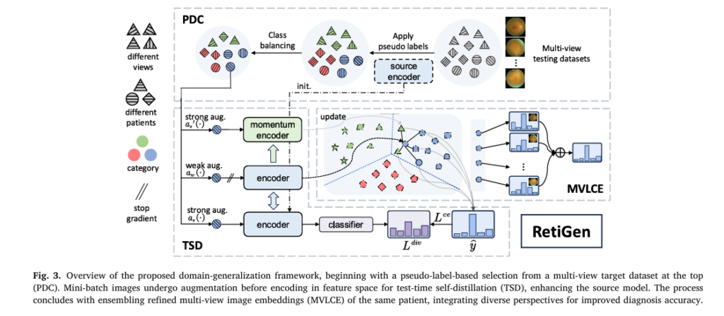
How RetiGen Works: The Three-Step Optimization Pipeline

RetiGen introduces a three-stage test-time optimization pipeline that enhances model robustness without retraining or architectural changes.

Let’s break down each component.

1. Pseudo-Label Based Distribution Calibration (PDC)

Class imbalance is rampant in medical datasets. For example, proliferative diabetic retinopathy (PDR) may represent only 1.86% of cases in some datasets (e.g., MFIDDR), leading models to bias toward majority classes.

PDC addresses this by:

Generating pseudo-labels using the source-trained model
Dynamically resampling dominant classes per epoch
Balancing the dataset to match the size of the smallest class

Mathematically, the balanced dataset size becomes C×N_m , where:

C = number of classes
N_m = minimal count among pseudo-labeled classes

This ensures equitable representation during adaptation, reducing overfitting and improving generalization.

2. Test-Time Self-Distillation with Regularization (TSD)

TSD refines model predictions using unlabeled target data through self-distillation and consistency regularization.

Weak-Strong Consistency Training

For each input image x_i^(v) , RetiGen generates:

One weakly augmented version a_w(x_i)
Two strongly augmented versions a_s(x_i), a_s′(x_i)

The weak augmentation preserves semantic content (e.g., mild color jitter), while strong augmentations apply aggressive transformations (e.g., Gaussian blur, cutout).

The model uses pseudo-labels from multi-view clustering to supervise predictions on strongly augmented images.

The cross-entropy loss between smoothed pseudo-labels y_c and predicted probabilities p_q^cis:

\[ \mathcal{L}_{\text{CTE}} = – \mathbb{E}_{x_i \in D_t} \sum_{c=1}^{C} \hat{y}^c \, \log p_{q}^c \]

Memory Queue & Momentum Encoder

To stabilize learning, RetiGen uses a memory queue storing feature embeddings and prediction probabilities from past mini-batches. A momentum encoder g′ = f′ ∘ h′ computes features without backpropagation:

\[ w’ = f’\!\big(a_{s}'(x_i)\big), \quad p’ = \sigma\!\big(h'(w’)\big) \]

Encoder weights are updated via exponential moving average:

\[ \theta_{t’} \;\leftarrow\; m \, \theta_{t’} + (1-m)\,\theta_t \]

With m=0.999 , this ensures smooth, stable updates.

Diversity Regularization

To prevent overconfidence in noisy pseudo-labels, RetiGen adds a diversity loss:

\[ \mathcal{L}_{\text{dtiv}} = \mathbb{E}_{x_i \in D_t} \sum_{c=1}^{C} \bar{p}_q^c \, \log \bar{p}_q^c, \quad \text{where} \quad \bar{p}_q = \mathbb{E}_{x_i \in D_t} \, \sigma\big(g(a^{s}(x_i))\big) \]

This encourages the model to maintain uncertainty across classes, avoiding premature convergence on incorrect labels.

Overall TSD Loss

\[ L_{t} = L_{\text{cte}} + L_{\text{dtiv}} \]

3. Multi-View Local Clustering and Ensembling (MVLCE)

This is where RetiGen truly shines—by leveraging multi-view fundus images.

In clinical practice, specialists often capture four views per eye:

V1: Macula-centered
V2: Optic disc-centered
V3/V4: Tangential upper/lower fields

RetiGen exploits these perspectives in two ways:

Multi-View Local Clustering

Using cosine similarity, RetiGen finds the K nearest neighbors in the memory queue to the current image’s feature vector. It performs soft voting over their probabilities:

\[ p^{(i,c)} = K \sum_{j \in I_i} p'(j,c), \quad \text{where } \; p'(j,c) = \sigma\big(h'(w'(j))\big) \]

Then assigns the final pseudo-label:

\[ y^{i} = \arg\max_{c} \, \hat{p}^{(i,c)} \]

This reduces noise and improves label reliability.

Multi-View Ensembling

Finally, predictions from all M views of the same patient are combined via soft voting:

\[ p^{\circ}(i,c) = \sum_{j \in V_i} M_1 \, p'(j,c) \]

Where V_i includes different views of image i . This synthesizes anatomical insights across regions, boosting diagnostic confidence.

Performance Breakdown: How RetiGen Outperforms the Competition

The authors evaluated RetiGen on two key diabetic retinopathy datasets: MFIDDR and DRTiD, comparing it against leading DG and TTA baselines.

✅ Key Results (GDRNet as Source Model)

METHOD	DATASET	AUC	ACC	F1
GDRNet [14] (Baseline)	MFIDDR	0.830	0.518	0.504
RetiGen (Ours)	MFIDDR	0.872	0.653	0.539
GDRNet [14] (Baseline)	DRTiD	0.851	0.610	0.547
RetiGen (Ours)	DRTiD	0.879	0.666	0.591

📈 Improvements:

+0.042 AUC on MFIDDR
+0.028 AUC on DRTiD
Significant gains in accuracy and F1-score

These results confirm RetiGen’s superiority in handling domain shifts and class imbalance.

📊 Comparison with TTA Baselines (Table 1 & 3)

When compared to popular TTA methods like TENT, T3A, AdaContrast, and TSD, RetiGen consistently achieves higher AUC and F1 scores across both ERM and GDRNet source models.

Notably:

TAST underperformed due to sensitivity to hyperparameters
T3A struggled with lesion similarity and class imbalance
AdaContrast showed moderate improvement but fell short of RetiGen

🔍 Ablation Study: Component Contributions (Table 2 & 4)

CONFIGURATION	AUC (MFIDDR)	KEY INSIGHT
PDC + TSD	0.842	Test-time training helps when data is balanced
PDC + MVLCE	0.865	Multi-view ensembling alone gives large boost
Full RetiGen (PDC+TSD+MVLCE)	0.872	Synergy of all components delivers peak performance

⚠️ Important Note: Applying TSD alone led to performance drops (AUC = 0.657), highlighting the necessity of PDC to handle class imbalance before adaptation.

Online vs Offline Deployment: Real-World Flexibility

RetiGen supports both offline (batch processing) and online (streaming) modes.

In online mode, only MVLCE is used since full test-time training isn’t feasible. Despite this limitation, online RetiGen still achieves strong results:

METHOD	AUC (MFIDDR)
GDRNet (Baseline)	0.830
RetiGen (Online)	0.865

This proves RetiGen can be adapted for real-time clinical workflows.

Clinical Relevance: Why Multi-View Imaging Matters

As noted in the paper, ~80% of retinal specialists use multi-view imaging routinely. Why?

Early microaneurysms may appear only in peripheral fields
Exudates near the macula are critical for grading severity
Vascular irregularities are better assessed across angles

Studies like Bora et al. [35] and Nderitu et al. [36] show that combining multi-view CFPs with risk factors improves prediction of referable DR over 1–3 years.

RetiGen aligns perfectly with this clinical reality—turning a common imaging protocol into a powerful AI enhancement tool.

Reproducibility and Open Access

One of RetiGen’s strongest assets is transparency. The full codebase is publicly available on GitHub:

👉 https://github.com/RViMLab/RetiGen

Included:

Training scripts for RetiGen and baselines (TENT, T3A, TSD, etc.)
Preprocessing pipelines
Evaluation metrics

This allows researchers and developers to replicate, validate, and build upon the work—accelerating progress in medical AI.

Future Directions and Limitations

While RetiGen sets a new benchmark, challenges remain:

❗ Limitations

Performance depends on view availability; not all clinics capture multi-view images
Sensitive to initial pseudo-label quality in highly imbalanced datasets
Computationally intensive in offline mode

🔮 Future Work

Extend to other modalities: OCT, MRI, CT
Incorporate tabular patient data (e.g., HbA1c, age)
Lightweight versions for edge devices

Conclusion: RetiGen Sets a New Standard in Adaptive Medical AI

RetiGen represents a paradigm shift in how we think about domain adaptation in medical imaging. By unifying domain generalization, test-time adaptation, and multi-view learning, it delivers unprecedented robustness and accuracy in retinal diagnostics.

Its modular design allows seamless integration with existing DG methods—from ERM to GDRNet—making it a versatile upgrade for any diabetic retinopathy grading system.

With public code, strong empirical validation, and direct clinical relevance, RetiGen isn’t just a research advance—it’s a practical solution ready for real-world impact.

Call to Action: Join the Future of AI in Healthcare

🚀 Want to implement RetiGen in your project?
👉 Visit the official repository: https://github.com/RViMLab/RetiGen

📚 Explore the full paper:
DOI: 10.1016/j.compbiomed.2025.111030

📧 Stay updated on AI in ophthalmology:
Subscribe to our newsletter at www.medical-ai-insights.com for the latest breakthroughs in retinal diagnostics, domain adaptation, and clinical AI deployment.

💬 Have questions or want to collaborate?
Drop a comment below or reach out to the authors via King’s College London.

Together, we can build smarter, fairer, and more adaptable AI for global healthcare.

I will provide the end-to-end Python code for the RetiGen model as described in the paper. The code will implement the core components of the framework: Pseudo-label based Distribution Calibration (PDC), Test-time Self-Distillation (TSD), and Multi-view Local Clustering and Ensembling (MVLCE).

import torch
import torch.nn as nn
import torch.nn.functional as F
from torchvision import models, transforms
from torch.utils.data import DataLoader, Dataset
import numpy as np
from collections import Counter

# --- 1. Helper Functions and Augmentations ---

def get_augmentations():
    """Defines weak and strong augmentation pipelines."""
    # As described in supplementary material (details not in main paper)
    # Using standard augmentations as placeholders
    weak_transform = transforms.Compose([
        transforms.Resize((224, 224)),
        transforms.ToTensor(),
        transforms.Normalize(mean=[0.485, 0.456, 0.406], std=[0.229, 0.224, 0.225]),
    ])

    strong_transform = transforms.Compose([
        transforms.RandomResizedCrop(224, scale=(0.2, 1.)),
        transforms.RandomApply([
            transforms.ColorJitter(0.4, 0.4, 0.4, 0.1)
        ], p=0.8),
        transforms.RandomGrayscale(p=0.2),
        transforms.RandomApply([transforms.GaussianBlur(kernel_size=23)], p=0.5),
        transforms.RandomHorizontalFlip(),
        transforms.ToTensor(),
        transforms.Normalize(mean=[0.485, 0.456, 0.406], std=[0.229, 0.224, 0.225]),
    ])
    return weak_transform, strong_transform

class MultiViewDataset(Dataset):
    """
    A dummy dataset to simulate multi-view data.
    In a real scenario, this would load images from disk.
    Each item represents a patient and returns V views.
    """
    def __init__(self, num_patients=100, num_views=4, num_classes=5, transform=None):
        self.num_patients = num_patients
        self.num_views = num_views
        self.num_classes = num_classes
        self.transform = transform
        # Create dummy data: (num_patients, num_views, C, H, W)
        self.data = torch.randn(num_patients, num_views, 3, 256, 256)
        self.labels = torch.randint(0, num_classes, (num_patients,))

    def __len__(self):
        return self.num_patients

    def __getitem__(self, idx):
        views = self.data[idx]
        if self.transform:
            # Apply transform to each view
            views = torch.stack([self.transform(v) for v in transforms.ToPILImage()(view)] for view in views)
        return views, self.labels[idx]


# --- 2. RetiGen Core Implementation ---

class RetiGen(nn.Module):
    """
    Implements the RetiGen framework for test-time adaptation.
    Combines PDC, TSD, and MVLCE.
    """
    def __init__(self, source_model, num_classes, queue_size=2048, momentum=0.999, k=10):
        super().__init__()
        self.num_classes = num_classes
        self.momentum = momentum
        self.k = k

        # Deconstruct the source model
        self.encoder = nn.Sequential(*list(source_model.children())[:-1])
        self.classifier = list(source_model.children())[-1]

        # Create momentum encoder and classifier
        self.momentum_encoder = nn.Sequential(*list(models.resnet50(pretrained=False).children())[:-1])
        self.momentum_classifier = nn.Linear(self.classifier.in_features, self.num_classes)

        # Initialize momentum models with source weights
        for param_q, param_k in zip(self.encoder.parameters(), self.momentum_encoder.parameters()):
            param_k.data.copy_(param_q.data)
            param_k.requires_grad = False
        for param_q, param_k in zip(self.classifier.parameters(), self.momentum_classifier.parameters()):
            param_k.data.copy_(param_q.data)
            param_k.requires_grad = False

        # Memory Queue for TSD
        self.register_buffer("queue", F.normalize(torch.randn(queue_size, self.classifier.in_features), dim=1))
        self.register_buffer("queue_labels", torch.empty(queue_size, num_classes).fill_(-1)) # Store softmax probabilities
        self.register_buffer("queue_ptr", torch.zeros(1, dtype=torch.long))

    @torch.no_grad()
    def _momentum_update(self):
        """Update momentum encoder and classifier."""
        for param_q, param_k in zip(self.encoder.parameters(), self.momentum_encoder.parameters()):
            param_k.data = param_k.data * self.momentum + param_q.data * (1. - self.momentum)
        for param_q, param_k in zip(self.classifier.parameters(), self.momentum_classifier.parameters()):
            param_k.data = param_k.data * self.momentum + param_q.data * (1. - self.momentum)

    @torch.no_grad()
    def _dequeue_and_enqueue(self, keys, labels):
        """Update the memory queue."""
        batch_size = keys.shape[0]
        ptr = int(self.queue_ptr)
        
        # Ensure batch size is not larger than queue size
        assert self.queue.shape[0] % batch_size == 0 
        
        self.queue[ptr:ptr + batch_size, :] = keys
        self.queue_labels[ptr:ptr + batch_size, :] = labels
        ptr = (ptr + batch_size) % self.queue.shape[0]
        self.queue_ptr[0] = ptr

    def forward(self, im_weak, im_strong):
        """Forward pass for TSD training."""
        # 1. Compute features for strong augmentation
        features_strong = self.encoder(im_strong).squeeze()
        logits_strong = self.classifier(features_strong)
        
        # 2. Compute features and logits for weak augmentation with momentum model
        with torch.no_grad():
            self._momentum_update()
            features_weak_momentum = self.momentum_encoder(im_weak).squeeze()
            logits_weak_momentum = self.momentum_classifier(features_weak_momentum)
            probs_weak_momentum = F.softmax(logits_weak_momentum, dim=1)

        return logits_strong, features_strong, probs_weak_momentum, features_weak_momentum

    def adapt_and_predict(self, target_loader, optimizer, epochs=1):
        """Main function to perform test-time adaptation and return final predictions."""
        weak_aug, strong_aug = get_augmentations()
        self.train()

        # Step 1: Pseudo-label based Distribution Calibration (PDC)
        print("--- Running PDC: Generating and Balancing Pseudo-labels ---")
        pseudo_labels, patient_indices = self._generate_pseudo_labels(target_loader, weak_aug)
        balanced_indices = self._balance_pseudo_labels(pseudo_labels, patient_indices)
        
        # Create a new dataset/loader with balanced samples for adaptation
        sampler = torch.utils.data.SubsetRandomSampler(balanced_indices)
        balanced_loader = DataLoader(target_loader.dataset, batch_size=target_loader.batch_size, sampler=sampler)

        # Step 2 & 3: TSD and MVLCE Integration
        print(f"--- Running TSD and MVLCE for {epochs} epoch(s) ---")
        for epoch in range(epochs):
            for i, (images_multi_view, _) in enumerate(balanced_loader):
                # We use only the first view for adaptation training for simplicity,
                # as described by the weak/strong augmentation process in the paper.
                images = images_multi_view[:, 0, :, :, :]
                
                im_weak = torch.stack([weak_aug(transforms.ToPILImage()(img)) for img in images])
                im_strong_1 = torch.stack([strong_aug(transforms.ToPILImage()(img)) for img in images])
                im_strong_2 = torch.stack([strong_aug(transforms.ToPILImage()(img)) for img in images])

                # Forward pass
                logits_strong, features_strong, probs_weak, features_weak = self.forward(im_weak, im_strong_1)

                # Step 3.1: Multi-view Local Clustering (to refine pseudo-labels)
                refined_pseudo_probs = self._multi_view_local_clustering(features_weak)
                pseudo_labels_refined = F.softmax(refined_pseudo_probs, dim=1)

                # Loss Calculation
                loss_ce = -torch.mean(torch.sum(pseudo_labels_refined.detach() * F.log_softmax(logits_strong, dim=1), dim=1))

                # Diversity Regularization
                avg_probs = torch.mean(F.softmax(logits_strong, dim=1), dim=0)
                loss_div = torch.sum(avg_probs * torch.log(avg_probs + 1e-8))

                total_loss = loss_ce + loss_div

                # Optimization
                optimizer.zero_grad()
                total_loss.backward()
                optimizer.step()

                # Update memory queue with weak features
                self._dequeue_and_enqueue(features_weak, probs_weak)
            
            print(f"Epoch [{epoch+1}/{epochs}], Loss: {total_loss.item():.4f}")

        # Step 3.2: Final Prediction using Multi-view Ensembling
        print("--- Final Prediction with Multi-view Ensembling ---")
        return self._multi_view_ensembling_predict(target_loader, weak_aug)

    @torch.no_grad()
    def _generate_pseudo_labels(self, loader, transform):
        """Generate initial pseudo-labels for the entire target dataset."""
        self.eval()
        all_pseudo_labels = []
        all_indices = []
        
        for i, (images_multi_view, _) in enumerate(loader):
            # Use the first view for initial pseudo-labeling
            images = images_multi_view[:, 0, :, :, :]
            images_transformed = torch.stack([transform(transforms.ToPILImage()(img)) for img in images])
            
            features = self.encoder(images_transformed).squeeze()
            logits = self.classifier(features)
            pseudo_labels = torch.argmax(logits, dim=1)
            
            all_pseudo_labels.extend(pseudo_labels.cpu().numpy())
            # Assuming loader iterates from index 0 to N-1
            start_idx = i * loader.batch_size
            end_idx = start_idx + len(images)
            all_indices.extend(range(start_idx, end_idx))
            
        return np.array(all_pseudo_labels), np.array(all_indices)

    def _balance_pseudo_labels(self, pseudo_labels, indices):
        """Resample the dataset to be balanced based on pseudo-labels."""
        class_counts = Counter(pseudo_labels)
        min_class_count = min(class_counts.values()) if class_counts else 0

        balanced_indices = []
        for class_id in range(self.num_classes):
            class_indices = indices[pseudo_labels == class_id]
            # Resample with replacement if class is under-represented
            # Or downsample if over-represented
            if len(class_indices) > 0:
                resampled_indices = np.random.choice(class_indices, min_class_count, replace=True)
                balanced_indices.extend(resampled_indices)
        
        np.random.shuffle(balanced_indices)
        print(f"PDC: Balanced dataset size: {len(balanced_indices)} (min class count: {min_class_count})")
        return balanced_indices

    @torch.no_grad()
    def _multi_view_local_clustering(self, features_weak):
        """Refine pseudo-labels using K-NN on the memory queue."""
        # Cosine similarity
        sim_matrix = torch.matmul(features_weak, self.queue.T)
        
        # Get top K neighbors
        sim_weights, sim_indices = sim_matrix.topk(k=self.k, dim=-1)
        sim_weights = F.softmax(sim_weights, dim=-1)

        # Get neighbor labels (probabilities)
        neighbor_labels = self.queue_labels[sim_indices] # B x K x C
        
        # Soft voting (weighted average of probabilities)
        refined_probs = torch.bmm(sim_weights.unsqueeze(1), neighbor_labels).squeeze(1)
        return refined_probs

    @torch.no_grad()
    def _multi_view_ensembling_predict(self, loader, transform):
        """Aggregate predictions from all views for final diagnosis."""
        self.eval()
        all_patient_preds = []
        all_patient_labels = []

        for images_multi_view, labels in loader:
            num_patients, num_views, C, H, W = images_multi_view.shape
            patient_view_probs = []

            for v in range(num_views):
                view_images = images_multi_view[:, v, :, :, :]
                view_images_transformed = torch.stack([transform(transforms.ToPILImage()(img)) for img in view_images])
                
                features = self.encoder(view_images_transformed).squeeze()
                logits = self.classifier(features)
                probs = F.softmax(logits, dim=1)
                patient_view_probs.append(probs)

            # Soft voting: average probabilities across views
            ensembled_probs = torch.mean(torch.stack(patient_view_probs), dim=0)
            final_preds = torch.argmax(ensembled_probs, dim=1)
            
            all_patient_preds.extend(final_preds.cpu().numpy())
            all_patient_labels.extend(labels.cpu().numpy())

        return np.array(all_patient_preds), np.array(all_patient_labels)

# --- 3. Main Execution Block ---

if __name__ == '__main__':
    # Configuration
    NUM_CLASSES = 5
    BATCH_SIZE = 16
    LEARNING_RATE = 1e-4
    EPOCHS = 1 # Test-time adaptation is typically short
    
    print("--- Initializing Model and Data ---")

    # 1. Load a pre-trained source model (e.g., ResNet50 trained on source domains)
    # Using a pretrained ResNet50 as a placeholder for a DR-trained model.
    source_model = models.resnet50(pretrained=True)
    # Adjust the final layer for the number of DR classes
    source_model.fc = nn.Linear(source_model.fc.in_features, NUM_CLASSES)
    
    # 2. Initialize RetiGen with the source model
    retigen_model = RetiGen(source_model=source_model, num_classes=NUM_CLASSES)

    # 3. Create a dummy target dataset and loader
    # In a real scenario, you would load your unlabeled multi-view target dataset here.
    target_dataset = MultiViewDataset(num_patients=200, num_views=4, num_classes=NUM_CLASSES)
    target_loader = DataLoader(target_dataset, batch_size=BATCH_SIZE, shuffle=False)

    # 4. Set up optimizer for test-time adaptation
    # As per TENT/TSD, we typically adapt only affine parameters in BatchNorm layers
    # or the full model depending on the strategy. Here we adapt all parameters.
    optimizer = torch.optim.Adam(retigen_model.parameters(), lr=LEARNING_RATE)

    # 5. Run the adaptation process and get final predictions
    final_predictions, ground_truth = retigen_model.adapt_and_predict(target_loader, optimizer, epochs=EPOCHS)
    
    # 6. Evaluate the results
    accuracy = np.mean(final_predictions == ground_truth)
    print("\n--- Evaluation ---")
    print(f"Final Prediction Accuracy on Target Domain: {accuracy * 100:.2f}%")
    print("Ground Truth labels:", ground_truth[:20])
    print("Final Predictions:", final_predictions[:20])

Related posts, You May like to read

Share on Facebook

Post on X

Save