The Plug-and-Play Module That Taught Neural Networks to Watch the Heart Move
A compact temporal attention module called TAM quietly outperforms much heavier architectures on cardiac segmentation — by making existing networks motion-aware without rebuilding them from scratch.
Every heartbeat is a small architectural event — walls contracting, valves opening, chambers cycling through a precisely orchestrated sequence. Cardiologists know this. They rely on motion to distinguish healthy tissue from pathological remodeling, to estimate ejection fraction, to catch the subtle asymmetries that precede heart failure. And yet, for years, deep learning models trained to segment cardiac anatomy have operated essentially frame-by-frame, treating each image as if the heart weren’t moving at all.
That mismatch has bothered researchers for a while. The fix — feeding image sequences into 3D or 4D convolutional networks — works in theory, but it turns out to be a practical headache. You need annotations for every frame, not just the easy-to-label end-diastole (ED) and end-systole (ES) timepoints that most clinical datasets provide. You need enormous GPU memory. And after all that computational investment, the improvements are often modest.
A team from Imperial College London’s Bioengineering Department — Md Kamrul Hasan, Guang Yang, and Choon Hwai Yap — has taken a different approach. Their paper, published in Medical Image Analysis in February 2026, proposes something called the Temporal Attention Module, or TAM: a small, modular operator that plugs into existing segmentation networks and gives them motion awareness for a fraction of the computational cost. The results, tested across four cardiac imaging datasets and six backbone architectures, are hard to dismiss.
Why Frame-by-Frame Segmentation Falls Short
Consider what a cardiologist actually sees when interpreting an echocardiogram. They’re not looking at 22 independent still images — they’re watching a loop, tracking how the left ventricle (LV) wall thickens during systole, how the myocardium (MYO) snaps back at diastole. That temporal context does a lot of perceptual work. Boundaries that look ambiguous in a single grainy ultrasound frame become clear when you watch them move for half a second.
Standard deep learning segmentation models — UNet, FCN8s, the more recent UNetR and SwinUNetR — don’t have that luxury. They process each frame in isolation. When speckle noise obscures the myocardial wall in frame 10, the model has no way of knowing what that region looked like in frames 8 or 9. Errors accumulate, and adjacent frames often produce segmentations that jump discontinuously — clinically nonsensical, and potentially dangerous when downstream measurements like ejection fraction depend on cross-frame consistency.
The obvious remedy is to add time as an explicit input dimension. Process frames together rather than one by one. Several research groups have done exactly this: Wei et al.’s CLAS network (2020) uses 3D convolutions for 2D+time echo sequences, while Myronenko et al. (2020) pushed it further with 4D convolutions for volumetric cardiac CT. Those approaches do help. But they also carry costs that become punishing at scale.
Adding the temporal dimension via 3D/4D convolutions increases FLOPs by as much as 8.5× and requires dense manual annotations across all time frames — a prohibitive constraint for 3D cardiac datasets, none of which currently provide complete temporal ground-truth segmentation.
Registration-based approaches try another angle: estimate the optical flow between frames, then use those motion fields to regularize segmentation. The SOCOF method (Xue et al., 2022) is a notable example. The idea is sound, but non-deep-learning registration is imperfect, and the resulting motion field errors can cascade into segmentation errors in exactly the cases — fast motion, large deformations — where you most need accuracy.
Temporal attention networks, like the multi-frame approach of Ahn et al. (2021) and the cross-attention approach of Wu et al. (2022), represent a more recent evolution. They compute attention between frames rather than concatenating them, which is more parameter-efficient. But these methods are baked into specific architectures. You can’t extract the temporal reasoning component and drop it into your existing model. That’s exactly the gap TAM was designed to fill.
The Core Idea: Motion Awareness as a Reusable Component
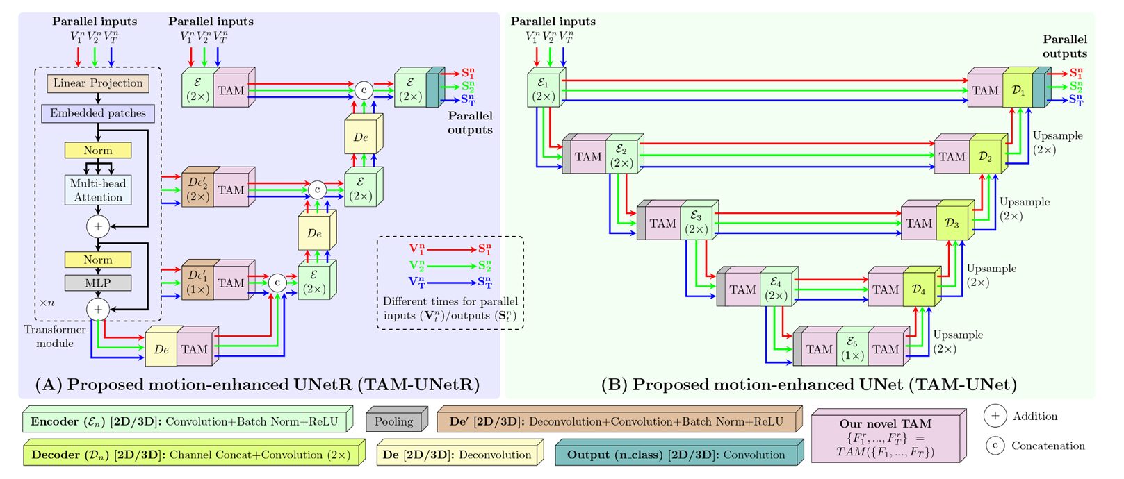
TAM is not a new architecture. That distinction matters. Rather than designing yet another segmentation network from scratch, Hasan and colleagues built a small, self-contained module that any segmentation network can absorb. Call it a cardiac motion adapter.
The module sits between two layers of a host network and takes in \(T\) feature maps — one per input frame — from the layer below. It then performs pairwise cross-temporal attention: for each target frame \(i\), it attends to every other reference frame \(j\) to figure out what motion-relevant information the reference frames carry that could help disambiguate the target frame. The refined feature maps are passed to the next layer. That’s it, structurally — but the devil, as always, is in the details of how that attention is computed and filtered.
Embedding Projections and Multi-Head Attention
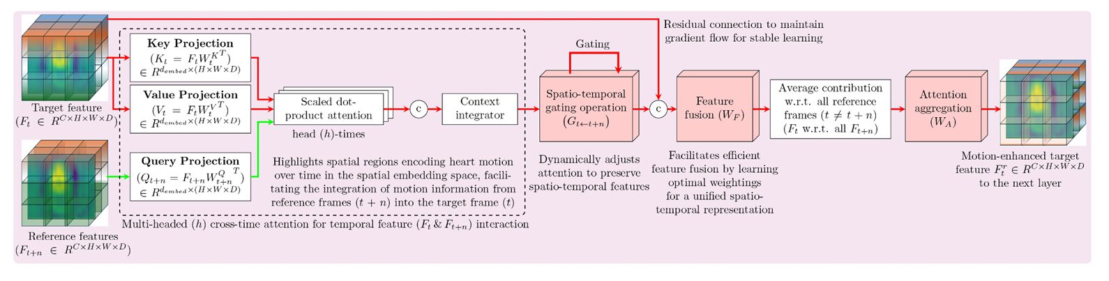
The module first projects the feature maps into Query, Key, and Value embeddings using learned weight matrices. Here, \(K_i\) and \(V_i\) represent the target frame, while \(Q_j\) represents the reference frames that seek relevant information from the target. The embeddings are split into \(H_\text{heads}\) subspaces — the same multi-head trick as in the original transformer (Vaswani, 2017) — enabling the network to simultaneously attend to different motion characteristics: slow versus fast displacements, simple versus complex boundary deformations.
The scaling factor \(\sqrt{d_\text{embed}/H_\text{heads}}\) stabilizes gradients, preventing the dot products from growing so large that the softmax saturates and attention collapses to a single position. This is standard transformer hygiene, but its inclusion here is what makes the attention numerically well-behaved even when processing low-contrast ultrasound frames with large regions of missing signal.
Spatio-Temporal Gating
This second component is what distinguishes TAM from simpler cross-frame attention designs. Not every cross-frame correlation is trustworthy. If one frame has a signal dropout artifact, the attention computed from that frame toward another carries noise. TAM addresses this with a learned gating function:
The sigmoid activation squashes gate values to \([0, 1]\), giving the model fine-grained control over how much information from each reference frame is preserved. Crucially, this gate is learned — it adapts through training to suppress unreliable regions and amplify motion-coherent anatomy. The Hadamard product (\(\odot\)) applies these scalar confidence scores element-wise to the attention output.
Feature Fusion and Temporal Aggregation
After gating, the target’s original feature map is concatenated with the gated attention output — a residual connection in spirit, borrowing from ResNet’s insight that shortcut paths stabilize gradient flow. A convolution followed by batch normalization and ReLU integrates the combined representation. Finally, motion features from all reference frames are averaged and passed through a \(1\times1\times1\) convolution to produce the refined target feature map:
The \(1\times1\times1\) convolution \(W_A\) learns a compact summary of the temporal consensus, compressing multiple reference-frame contributions into a single refined representation of the target frame.
“TAM’s novelty lies in decoupling temporal modeling from network construction — enabling cross-time interaction at different semantic levels, and explicitly modeling temporal reliability through spatio-temporal gating.” — Hasan, Yang & Yap, Medical Image Analysis, 2026
Sparse Supervision: The Practical Advantage Nobody Talks About Enough
Here’s a constraint that anyone who has worked on cardiac segmentation knows intimately. Annotating full cardiac cycles is miserable work. For 2D echo sequences, annotators must label 15–25 frames per patient. For 3D sequences — volumes evolving over time — that burden becomes nearly prohibitive. Ensuring inter-slice consistency in 3D manual annotations is genuinely hard; the resulting ground truths are often anatomically implausible without additional post-processing.
Most clinical cardiac datasets compromise. The ACDC 3D MRI dataset, for instance, provides manual annotations only at ED and ES — the two most clinically meaningful timepoints. Everything in between is unannotated. This is actually the norm, not the exception.
TAM handles this gracefully. During training, the loss function — a combination of Dice coefficient and cross-entropy, summed over available annotated frames — does not require labels at every temporal position:
where \(T’ \leq T\) is the subset of frames with available annotations. Even with \(T’ = 2\) (just ED and ES), the unlabeled intermediate frames still contribute motion context through TAM’s attention mechanism — the network learns temporal dynamics from the intensity images, even when no label is available for those frames.
The experiments confirm this works. Comparing sparse supervision (ED+ES labels only) against dense supervision (all frames labeled) shows that the DSC difference is negligible, with HD improvements from adding more labels that are not statistically significant beyond certain frame counts. That’s a meaningful result for clinical translation: you don’t need a labeling army to train a temporally aware model.
TAM achieves motion-aware segmentation with as few as two annotated frames per cardiac cycle. Dense temporal annotation — one of the most time-consuming bottlenecks in cardiac AI dataset creation — is no longer required.
The Architecture of Restraint: Why Smaller TAM Configurations Win
One of the more counterintuitive findings in the ablation study involves where to place TAM within a host network. The authors tested nine configurations (C3–C11) varying insertion points across encoder layers 3 and 4, the bottleneck layer 5, and decoder layers 3 and 4. The expectation might be that more TAM is better — more temporal attention at more levels means richer motion information, right?
Not quite. Performance is largely similar across all configurations, while FLOPs and parameter counts grow steadily with each additional TAM insertion. The C4 configuration — TAM at layers 4 and 5 only — emerges as the practical sweet spot, achieving excellent performance with 228G FLOPs and 62M parameters. Compare that to the baseline UNet3D (2D+t) with ED and ES frames: 560G FLOPs, 87M parameters, and actually worse HD performance than C4.
| Model | DSC ↑ | HD (mm) ↓ | MASD (mm) ↓ | FLOPs ↓ | Params ↓ |
|---|---|---|---|---|---|
| UNet2D (frame-by-frame, no motion) | 0.913 | 5.11 | 1.13 | 193G | 31M |
| UNet3D (2D+t, ED & ES only) | 0.915 | 5.65 | 1.15 | 560G | 87M |
| UNet3D (2D+t, all 17 frames) | 0.917 | 4.92 | 1.09 | 4764G | 87M |
| TAM-UNet2D, C4 (ED & ES) | 0.922 | 3.63 | 0.961 | 228G | 62M |
| TAM-UNet2D, C5 (ED & ES) | 0.923 | 3.51 | 0.954 | 237G | 66M |
Results on the 2D CAMUS dataset (Leclerc et al., 2019). C4 and C5 use TAM at encoder layers 4–5 (±layer 3). All TAM configurations use 8 attention heads. Independent t-test significance (p < .05) confirmed for all TAM vs. UNet2D comparisons.
The computational argument is crisp: the 3D UNet that processes all 17 frames needs 4764G FLOPs — twenty-five times more computation than TAM-UNet C4 — to achieve a DSC of 0.917 and HD of 4.92 mm. TAM-UNet C4, with just two frames as input, hits 0.922 DSC and 3.63 mm HD. The attention mechanism extracts more actionable temporal information from fewer frames than brute-force temporal convolution.
Why does attention win here? Because what matters is not the quantity of frames, but the quality of the comparison between them. ED and ES are maximally dissimilar cardiac states — peak relaxation versus peak contraction. The attention mechanism finds exactly what distinguishes these two states spatially, which is precisely what you need to understand the deformation field and produce motion-coherent segmentations.
Cross-Architecture Generalization: Plugging Into Everything
One claim that’s easy to make and hard to prove is true architecture-agnosticism. The team ran TAM across six different backbones: UNet, FCN8s, UNetR, SwinUNetR, I²UNet (Dai et al., 2024), and DT-VNet (Cai et al., 2024). Every single one improved across all four metrics after TAM integration, tested on both 2D (CAMUS, EchoNet-Dynamic) and 3D (MITEA echocardiography, ACDC MRI) datasets.
That’s not nothing. The performance gains aren’t uniform — CNN backbones like UNet and FCN8s benefit more dramatically than transformer-based ones like SwinUNetR. The explanation is sensible: transformers already incorporate global context through self-attention, so some of TAM’s contribution overlaps with what the backbone does anyway. With CNN networks, whose receptive fields are inherently local and spatially bounded, TAM’s cross-frame global reasoning fills a genuine gap.
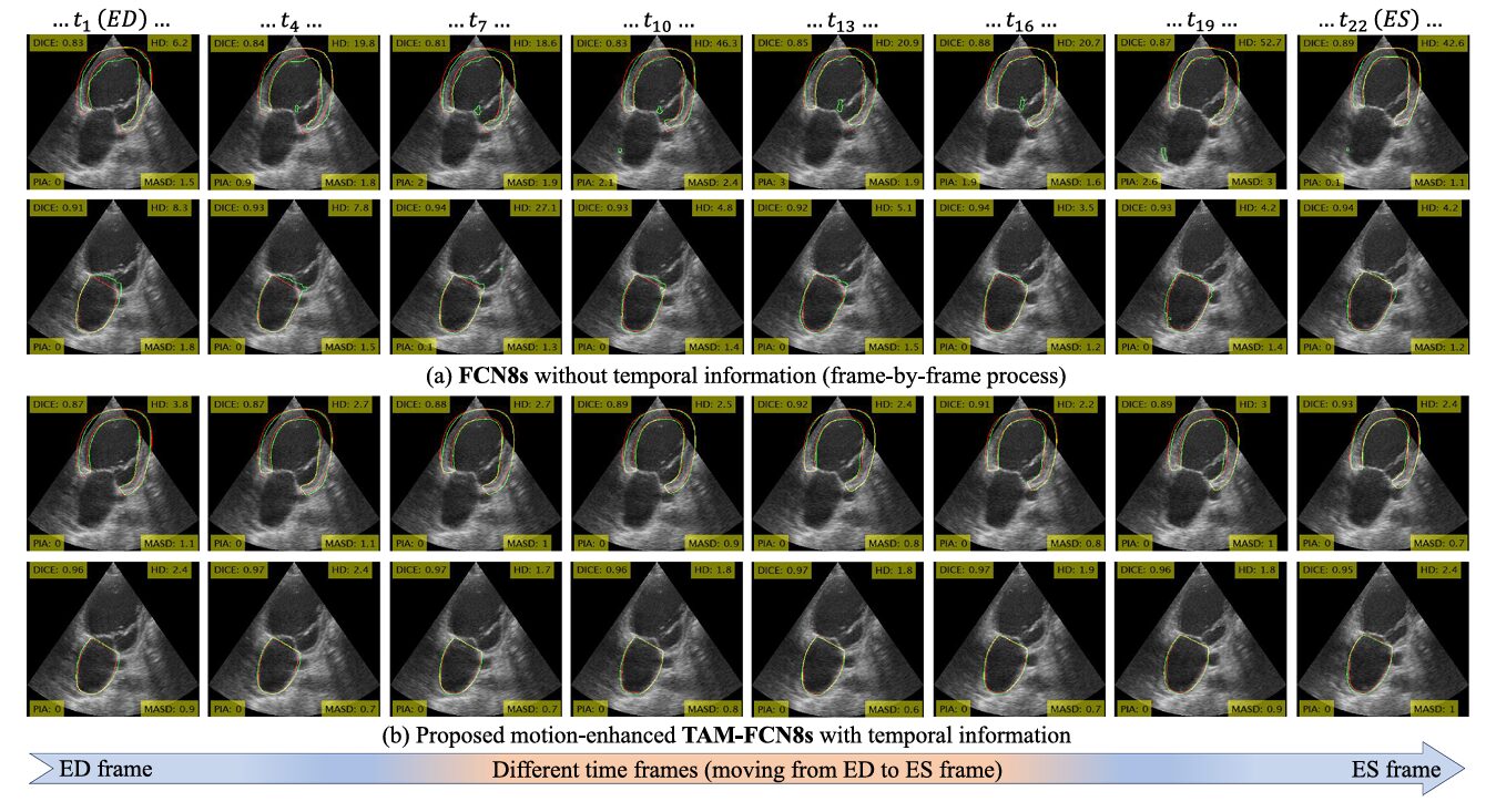
The Hausdorff distance (HD) improvements tell the clearest story. HD measures the worst-case boundary error — the maximum distance between any predicted boundary point and the nearest ground-truth point. It’s a harsh metric, punishing exactly the kind of catastrophic failure that makes clinical deployment risky. TAM’s integration into FCN8s on the CAMUS dataset cuts HD from 6.38 mm to 3.31 mm, a 48% reduction. That’s not an incremental improvement — it’s the difference between a segmentation that’s occasionally dangerously wrong and one that maintains much more uniform boundary accuracy.
TAM and the Percentage of Island Area Metric
The authors introduce a custom evaluation metric called PIA — Percentage of Island Area — that deserves attention. Standard DSC scores can look acceptable even when a segmentation produces anatomically implausible disconnected regions, because those isolated islands might still overlap substantially with ground truth. PIA directly quantifies this failure mode by measuring the total area of disconnected regions relative to the largest segmented component, without requiring ground truth.
TAM’s effect on PIA is sometimes more dramatic than its effect on DSC. For FCN8s on the CAMUS dataset, integrating TAM drops PIA from 0.58% to 0.02% — a near-total elimination of segmentation islands. On the 3D MITEA dataset, the same pairing reduces PIA from 1.07% to 0.22%. These improvements are not cosmetic; isolated segmentation islands produce erroneous volume measurements and incorrect shape reconstructions that propagate into downstream clinical metrics.
Extending to SAM and MedSAM: Temporal Prompting
One of the more creative experiments in the paper couples TAM with the Segment Anything Model (SAM, Kirillov et al., 2023) and its medical imaging variant MedSAM (Ma et al., 2024). SAM is an interactive segmentation model — you give it a spatial prompt (a bounding box, say), and it segments the indicated object. The model was trained on a vast natural image corpus and shows impressive zero-shot generalization.
The problem for cardiac sequences is that SAM is static. You’d need to provide a bounding box for every frame, which defeats much of the convenience. The team’s TAM-SAM variant adds a prompt encoder at the bottleneck of SAM’s encoder and propagates a single bounding box prompt across the entire sequence through TAM’s temporal attention. The result is motion-aware interactive segmentation: annotate one frame, get temporally consistent segmentations for the whole cycle.
On the CAMUS dataset, TAM-SAM reduces HD from 3.99 mm (vanilla SAM) to 3.51 mm — statistically significant at p < 0.05. On EchoNet-Dynamic, fine-tuned TAM-MedSAM achieves an HD of 2.06 pixels versus 3.04 for fine-tuned MedSAM alone, and surpasses recent state-of-the-art echo segmentation methods including EchoSAM (Li et al., 2025) and NCM-Net (Deng & Wu, 2025).
Clinical Relevance: Ejection Fraction as the Ground Truth Test
Segmentation accuracy metrics — DSC, HD, MASD — are proxies. What clinicians care about is whether the model’s outputs lead to better clinical measurements. The most important single metric in cardiac function assessment is ejection fraction: the percentage of blood pumped out of the left ventricle with each beat. EF below 40% triggers heart failure diagnoses and treatment decisions. Errors in segmentation propagate directly into EF estimation errors.
The authors tested EF estimation using the regression correlation between model-predicted and ground-truth EF values. Baseline UNet achieves a correlation of 87.9%. Adding the multi-frame temporal attention approach of Ahn et al. (2021) pushes it to 90.6%. TAM-UNet reaches 92.25% — the best performance among all compared methods, including optical flow-based SOCOF (89.3%). The MSE drops from 50.0 to 29.0 across the same comparisons.
This is where the clinical story comes together. More consistent cross-frame segmentations mean more reliable volume estimates at ED and ES, which means smaller EF estimation errors, which means fewer misclassified patients at the diagnostic threshold. These improvements have real stakes.
Results at Scale: 3D Echocardiography and Cardiac MRI
Scaling from 2D to 3D introduces additional complexity that tests TAM’s design claims. 3D cardiac images have sparser regions of interest relative to image volume, more anatomical complexity per sample, and fewer available ground-truth annotations per dataset — all conspiring to make the segmentation problem harder.
On the 3D MITEA echocardiography dataset (134 patients, 536 volumes), TAM-FCN8s achieves a statistically significant HD reduction from 11.66 mm to 8.37 mm. On the 3D ACDC cardiac MRI dataset, TAM-UNet produces an average DSC of 0.931 against UNet’s 0.924, with HD dropping from 7.52 mm to 4.43 mm. These gains are consistent across CNN, transformer, and hybrid backbones.
The 3D visualizations from ACDC are striking. Without TAM, 3D reconstructions of cardiac chambers show isolated misclassified voxel clusters — surface protrusions that violate anatomical plausibility. With TAM, those artifacts are suppressed, and cavity shapes are more complete and coherent. Motion context, even summarized from just ED and ES frames, is sufficient to guide the network toward anatomically reasonable 3D reconstructions.
One comparison stands out in the 3D ACDC benchmark. TAM-UNet’s average DSC of 0.931 edges out the recent UNetR++ (0.928) and nnFormer (0.921) — two purpose-built state-of-the-art architectures — using a much simpler base network augmented only with TAM. The implication is uncomfortable for the trend toward ever-more-complex architectures: a small, well-designed motion module on a simple foundation can beat elaborate monolithic models that ignore temporal context.
| Method | Backbone | DSC ↑ | HD mm ↓ | Temporal? |
|---|---|---|---|---|
| nnFormer (Zhou et al., 2023) | Transformer | 0.921 | — | ✗ |
| UNetR++ (Shaker et al., 2024) | Transformer | 0.928 | — | ✗ |
| DT-VNet (Cai et al., 2024) | Hybrid | 0.914 | 6.83 | ✗ |
| TAM-DT-VNet (ours) | Hybrid + TAM | 0.920 | 5.19 | ✓ |
| TAM-UNet (ours) | CNN + TAM | 0.931 | 4.43 | ✓ |
Comparison on the 3D ACDC cardiac MRI dataset. Average over LV myocardium, LV endocardium, and right ventricle. TAM-UNet outperforms all compared methods in both DSC and HD.
What TAM Doesn’t Yet Solve
The authors are candid about the limitations, which is worth acknowledging. The current design assumes temporally regular input sampling — frames at consistent intervals. That assumption may not hold for real-time acquisitions with vendor-specific frame rate variations, or for scans disrupted by patient movement or arrhythmias. Incorporating learnable temporal encodings that adapt to irregular sampling is an obvious next step, and not a trivial one.
There’s also the question of clinical pathological diversity. The datasets here — CAMUS, EchoNet-Dynamic, MITEA, ACDC — span normal subjects and common pathologies. But cardiac anatomy in severe congenital anomalies or complex cardiomyopathies can look profoundly different from the training distribution. TAM’s motion priors, learned from relatively standard cardiac cycles, may not generalize as cleanly to atypical motion patterns.
The 2D versus 3D performance gap also warrants caution. TAM’s absolute HD improvements tend to be larger in 2D than 3D, partly because 3D segmentation baselines are already stronger relative to the task difficulty, and partly because the per-voxel attention becomes more diffuse as spatial dimensions grow. Scaling strategies — perhaps hierarchical attention or resolution-adaptive gating — may be needed to maintain efficiency as volumetric resolution increases.
What This Work Actually Means
The central achievement here is not a performance number, though the performance numbers are good. It’s a design philosophy vindicated by experiment: you do not need to redesign a segmentation network to make it temporally aware. You need to build a reusable, well-engineered temporal operator and let it do its job inside whatever backbone you’re already using. TAM’s consistent improvement across six backbone architectures, four datasets, and two modalities (echocardiography and MRI) is strong evidence that this philosophy scales.
There’s a conceptual shift embedded in that result worth sitting with. The field has spent years arguing about which segmentation architecture is best — UNet versus transformer, CNN versus hybrid. TAM’s success with something as simple as FCN8s, where it outperforms fancier architectures without TAM, suggests we’ve been arguing about the wrong thing. What the heart needs from a deep learning model is not global self-attention, or dilated convolutions, or multi-scale feature pyramids per se. It needs to understand that anatomy moves — and that understanding motion, even crudely, from two well-chosen frames, is more diagnostic than any amount of spatial sophistication applied to a single snapshot.
The transferability of this insight extends well beyond cardiac imaging. TAM’s design makes no assumptions specific to the heart. The attention mechanism cares only that features vary meaningfully across time and that learning to compare them will improve predictions. Tumor progression monitoring in 4D CT, liver motion analysis in cine MRI, airway wall tracking in pulmonary imaging — any domain where anatomy deforms and existing models operate frame-by-frame is a potential application. The plug-and-play design means adoption is low-friction: integrate TAM at the encoder bottleneck, train with the available sparse labels, and observe whether performance improves. In most cases, based on what we see here, it will.
Honestly, the sparse annotation finding may be the most practically important contribution. The annotation bottleneck is arguably the largest single obstacle to deploying cardiac AI in clinical settings. If you need ground truth for every frame of every cardiac cycle, your labeling costs scale linearly with the temporal resolution of your dataset. TAM breaks that coupling. Two annotated frames per patient — the ED/ES pair that every major cardiac dataset already provides — are sufficient. That turns a labeling problem that required specialized cardiologist time for every frame into one that requires exactly the annotation effort that has already been done.
Future work should push in a few directions that the authors outline. LoRA-style integration of TAM into large foundation models like MedSAM could enable efficient multi-modal adaptation without full fine-tuning. Multi-task extensions — joint segmentation and motion quantification — could produce clinically richer outputs from a single inference pass. And continual learning frameworks that allow TAM-equipped models to update their motion priors as they encounter new pathologies could eventually support deployment in settings where the case mix evolves over time.
The deeper lesson here is one about engineering humility. A 31-million-parameter UNet, augmented with a 31-million-parameter TAM module and trained on two labeled frames per patient, outperforms architectures three times its size trained on full-sequence annotations. Complexity is not the same as capability. Knowing what to look at — and when — remains more valuable than the ability to look at everything at once.
Complete Proposed Model Code (PyTorch)
The implementation below faithfully reproduces TAM as described in the paper, including the multi-head cross-temporal attention mechanism, spatio-temporal gating, feature fusion, and temporal aggregation. It maps directly to Algorithm 2 in Appendix A, integrates TAM into a standard UNet2D backbone (the C4 configuration from Table 1), and includes the spatio-temporal loss function from Equation 1. A runnable smoke test at the bottom validates the forward pass with dummy 2D+time cardiac data.
# ─────────────────────────────────────────────────────────────────────────────
# TAM: Temporal Attention Module for Motion-Guided Cardiac Segmentation
# Hasan, Yang & Yap · Medical Image Analysis 2026
# Full PyTorch implementation: TAM core, TAM-UNet2D (C4), loss, train & eval
# ─────────────────────────────────────────────────────────────────────────────

import torch
import torch.nn as nn
import torch.nn.functional as F
from torch.optim import Adam
import numpy as np


# ─── Section 1: Temporal Attention Module (TAM) Core ─────────────────────────

class TemporalAttentionModule(nn.Module):
    """
    TAM: plug-and-play cross-temporal attention with spatio-temporal gating.

    Receives T feature maps from the previous network layer and returns T
    motion-enhanced feature maps of identical shape.

    Args:
        channels   : Number of feature channels C (spatial dimension of feature map).
        d_embed    : Embedding dimension for Q/K/V projections.
        n_heads    : Number of attention heads H_heads. Paper uses 8.
        spatial_dim: Tuple (H, W) for 2D or (H, W, D) for 3D feature maps.
    """

    def __init__(self, channels: int, d_embed: int = 64,
                 n_heads: int = 8):
        super().__init__()
        self.n_heads = n_heads
        self.d_embed = d_embed
        self.scale   = (d_embed // n_heads) ** -0.5

        # ── Q / K / V linear projections (shared across all frames) ──────────
        self.W_q = nn.Linear(channels, d_embed, bias=True)
        self.W_k = nn.Linear(channels, d_embed, bias=True)
        self.W_v = nn.Linear(channels, d_embed, bias=True)

        # ── Context integrator: fuse multi-head output back to d_embed ────────
        self.context_proj = nn.Linear(d_embed, d_embed, bias=True)

        # ── Spatio-temporal gating convolution (applied per spatial position) ─
        self.gate_conv = nn.Conv2d(d_embed, d_embed, kernel_size=1)

        # ── Feature fusion: concat(F_i, A_gated) → conv → BN → ReLU ─────────
        self.fusion = nn.Sequential(
            nn.Conv2d(channels + d_embed, channels, kernel_size=1),
            nn.BatchNorm2d(channels),
            nn.ReLU(inplace=True),
        )

        # ── Attention aggregation: 1×1 conv over averaged temporal features ───
        self.agg_conv = nn.Conv2d(channels, channels, kernel_size=1)

    def _project_qkv(self, feat_map: torch.Tensor):
        """
        Reshape feature map for multi-head attention computation.

        Args:
            feat_map: [B, C, H, W]
        Returns:
            Q, K, V: each [B, n_heads, H*W, d_head]
        """
        B, C, H, W = feat_map.shape
        x_flat = feat_map.permute(0, 2, 3, 1).reshape(B, H * W, C)  # [B, N, C]

        Q = self.W_q(x_flat)  # [B, N, d_embed]
        K = self.W_k(x_flat)
        V = self.W_v(x_flat)

        d_head = self.d_embed // self.n_heads
        # Reshape to [B, n_heads, N, d_head] for batched matmul
        Q = Q.reshape(B, H * W, self.n_heads, d_head).permute(0, 2, 1, 3)
        K = K.reshape(B, H * W, self.n_heads, d_head).permute(0, 2, 1, 3)
        V = V.reshape(B, H * W, self.n_heads, d_head).permute(0, 2, 1, 3)
        return Q, K, V, H, W

    def _cross_temporal_attention(self, Q_j, K_i, V_i):
        """
        Compute cross-temporal attention A^h_{i←j} for all heads.

        A = softmax(Q_j · K_i^T / sqrt(d_head)) · V_i

        Args:
            Q_j, K_i, V_i: each [B, n_heads, N, d_head]
        Returns:
            attn_out: [B, n_heads, N, d_head]
        """
        scores = torch.matmul(Q_j, K_i.transpose(-2, -1)) * self.scale  # [B, H, N, N]
        attn_weights = F.softmax(scores, dim=-1)
        return torch.matmul(attn_weights, V_i)   # [B, H, N, d_head]

    def forward(self, features: list[torch.Tensor]) -> list[torch.Tensor]:
        """
        Forward pass over T feature maps.

        Args:
            features: List of T tensors, each [B, C, H, W]
        Returns:
            refined:  List of T motion-enhanced tensors, each [B, C, H, W]
        """
        T  = len(features)
        B, C, H, W = features[0].shape
        N  = H * W

        # ── Pre-project all frames ────────────────────────────────────────────
        projs = [self._project_qkv(f) for f in features]
        # projs[t] = (Q_t, K_t, V_t, H, W)   each Q/K/V: [B, n_heads, N, d_head]

        refined = []

        for i in range(T):
            Q_i, K_i, V_i, _, _ = projs[i]
            F_i = features[i]                # [B, C, H, W] — original target feature

            pairwise_fused = []

            for j in range(T):
                if j == i:
                    continue

                Q_j, _, _, _, _ = projs[j]

                # ── Step 1: Multi-head cross-temporal attention ───────────────
                A_h = self._cross_temporal_attention(Q_j, K_i, V_i)
                # Concat heads: [B, n_heads, N, d_head] → [B, N, d_embed]
                A_multi = A_h.permute(0, 2, 1, 3).reshape(B, N, self.d_embed)
                A_multi = self.context_proj(A_multi)                   # [B, N, d_embed]
                A_multi = A_multi.permute(0, 2, 1).reshape(B, self.d_embed, H, W)
                # Now: [B, d_embed, H, W]

                # ── Step 2: Spatio-temporal gating ───────────────────────────
                G     = torch.sigmoid(self.gate_conv(A_multi))         # [B, d_embed, H, W]
                A_gated = A_multi * G                                   # element-wise

                # ── Step 3: Feature fusion (skip connection) ──────────────────
                combined = torch.cat([F_i, A_gated], dim=1)            # [B, C+d_embed, H, W]
                F_fused  = self.fusion(combined)                        # [B, C, H, W]
                pairwise_fused.append(F_fused)

            # ── Step 4: Temporal averaging + 1×1 aggregation conv ─────────────
            F_avg = torch.stack(pairwise_fused, dim=0).mean(dim=0)     # [B, C, H, W]
            F_r   = self.agg_conv(F_avg)                                # [B, C, H, W]
            refined.append(F_r)

        return refined


# ─── Section 2: UNet Building Blocks ─────────────────────────────────────────

class ConvBlock(nn.Module):
    """Double convolution block: Conv→BN→ReLU × 2."""

    def __init__(self, in_ch, out_ch):
        super().__init__()
        self.block = nn.Sequential(
            nn.Conv2d(in_ch,  out_ch, 3, padding=1, bias=False),
            nn.BatchNorm2d(out_ch), nn.ReLU(inplace=True),
            nn.Conv2d(out_ch, out_ch, 3, padding=1, bias=False),
            nn.BatchNorm2d(out_ch), nn.ReLU(inplace=True),
        )

    def forward(self, x):
        return self.block(x)


class UpBlock(nn.Module):
    """Upsample by 2 then fuse skip connection."""

    def __init__(self, in_ch, skip_ch, out_ch):
        super().__init__()
        self.up   = nn.Upsample(scale_factor=2, mode="bilinear", align_corners=True)
        self.conv = ConvBlock(in_ch + skip_ch, out_ch)

    def forward(self, x, skip):
        x = self.up(x)
        # Handle spatial size mismatch from pooling
        dH = skip.shape[2] - x.shape[2]
        dW = skip.shape[3] - x.shape[3]
        x  = F.pad(x, [dW // 2, dW - dW // 2, dH // 2, dH - dH // 2])
        return self.conv(torch.cat([skip, x], dim=1))


# ─── Section 3: TAM-UNet2D (C4 configuration) ────────────────────────────────

class TAMUNet2D(nn.Module):
    """
    TAM-UNet2D — C4 configuration from Table 1 (Hasan et al., 2026).

    TAM is inserted at encoder depth-4 (enc4) and the bottleneck (enc5).
    Accepts T frames in parallel and produces T segmentation masks.

    Args:
        in_channels : Image channels (1 for grayscale echo, 3 for RGB).
        n_classes   : Number of segmentation classes (e.g. 4 for CAMUS).
        base_ch     : Base channel count, doubled at each encoder depth.
        T           : Number of temporal frames (2 for ED+ES, 3 with mid-frame).
        tam_d_embed : Embedding dimension for TAM projections.
        tam_heads   : Number of attention heads in TAM (paper: 8).
    """

    def __init__(
        self,
        in_channels: int = 1,
        n_classes:   int = 4,
        base_ch:     int = 32,
        T:           int = 2,
        tam_d_embed: int = 64,
        tam_heads:   int = 8,
    ):
        super().__init__()
        self.T = T
        ch = [base_ch, base_ch * 2, base_ch * 4, base_ch * 8, base_ch * 16]

        # ── Encoder ─────────────────────────────────────────────────────────
        self.enc1 = ConvBlock(in_channels, ch[0])   # depth 1 → 256×256
        self.enc2 = ConvBlock(ch[0], ch[1])         # depth 2 → 128×128
        self.enc3 = ConvBlock(ch[1], ch[2])         # depth 3 → 64×64
        self.enc4 = ConvBlock(ch[2], ch[3])         # depth 4 → 32×32
        self.enc5 = ConvBlock(ch[3], ch[4])         # bottleneck → 16×16
        self.pool = nn.MaxPool2d(2)

        # ── TAM modules (C4: enc4 and enc5) ─────────────────────────────────
        self.tam4 = TemporalAttentionModule(ch[3], tam_d_embed, tam_heads)
        self.tam5 = TemporalAttentionModule(ch[4], tam_d_embed, tam_heads)

        # ── Decoder ─────────────────────────────────────────────────────────
        self.dec4 = UpBlock(ch[4], ch[3], ch[3])
        self.dec3 = UpBlock(ch[3], ch[2], ch[2])
        self.dec2 = UpBlock(ch[2], ch[1], ch[1])
        self.dec1 = UpBlock(ch[1], ch[0], ch[0])
        self.out  = nn.Conv2d(ch[0], n_classes, kernel_size=1)

    def forward(self, frames: list[torch.Tensor]) -> list[torch.Tensor]:
        """
        Process T parallel input frames and return T segmentation logits.

        Args:
            frames: List of T tensors, each [B, in_channels, H, W].
        Returns:
            masks:  List of T tensors, each [B, n_classes, H, W].
        """
        assert len(frames) == self.T

        # ── Encode each frame independently through depths 1–3 ───────────────
        e1s, e2s, e3s, e4s, e5s = [], [], [], [], []

        for x in frames:
            e1 = self.enc1(x)                   # [B, ch0, H,    W   ]
            e2 = self.enc2(self.pool(e1))        # [B, ch1, H/2,  W/2 ]
            e3 = self.enc3(self.pool(e2))        # [B, ch2, H/4,  W/4 ]
            e4 = self.enc4(self.pool(e3))        # [B, ch3, H/8,  W/8 ]
            e5 = self.enc5(self.pool(e4))        # [B, ch4, H/16, W/16]
            e1s.append(e1); e2s.append(e2); e3s.append(e3)
            e4s.append(e4); e5s.append(e5)

        # ── Apply TAM at depth 4 (C4 configuration) ─────────────────────────
        e4s_r = self.tam4(e4s)      # refined cross-frame features at encoder depth 4

        # ── Apply TAM at bottleneck depth 5 ─────────────────────────────────
        e5s_r = self.tam5(e5s)      # refined cross-frame features at bottleneck

        # ── Decode each frame using its refined features ─────────────────────
        outputs = []
        for t in range(self.T):
            d4 = self.dec4(e5s_r[t], e4s_r[t])
            d3 = self.dec3(d4, e3s[t])
            d2 = self.dec2(d3, e2s[t])
            d1 = self.dec1(d2, e1s[t])
            outputs.append(self.out(d1))

        return outputs


# ─── Section 4: Spatio-Temporal Loss (Equation 1) ────────────────────────────

def dice_loss(pred: torch.Tensor, target: torch.Tensor, eps: float = 1e-6) -> torch.Tensor:
    """
    Soft Dice loss over all classes (macro-averaged).

    Args:
        pred   : [B, C, H, W] — raw logits.
        target : [B, H, W]    — integer class labels.
        eps    : Numerical stability constant.
    Returns:
        Scalar Dice loss.
    """
    n_classes = pred.shape[1]
    pred_soft = F.softmax(pred, dim=1)                         # [B, C, H, W]
    tgt_one   = F.one_hot(target, n_classes).permute(0, 3, 1, 2).float()

    intersection = (pred_soft * tgt_one).sum(dim=(0, 2, 3))     # [C]
    union        = pred_soft.sum(dim=(0, 2, 3)) + tgt_one.sum(dim=(0, 2, 3))
    dice_per_cls = (2 * intersection + eps) / (union + eps)     # [C]
    return 1 - dice_per_cls.mean()


def ce_loss(pred: torch.Tensor, target: torch.Tensor) -> torch.Tensor:
    """Standard cross-entropy loss for multi-class segmentation."""
    return F.cross_entropy(pred, target)


def spatio_temporal_loss(
    preds:   list[torch.Tensor],
    targets: list[torch.Tensor | None],
    lam_dice: float = 0.5,
    lam_ce:   float = 0.5,
) -> torch.Tensor:
    """
    Spatio-temporal loss L from Equation 1 (Hasan et al., 2026).

    Supports sparse temporal supervision: frames where target is None
    are skipped, so the loss is computed only over annotated frames.

    Args:
        preds   : List of T prediction tensors [B, C, H, W].
        targets : List of T target tensors [B, H, W] or None (unlabelled).
        lam_dice: Weight for Dice component.
        lam_ce  : Weight for cross-entropy component.
    Returns:
        Scalar spatio-temporal loss, averaged over annotated frames T'.
    """
    annotated_losses = []

    for pred, tgt in zip(preds, targets):
        if tgt is None:
            continue               # skip unannotated frames — sparse supervision
        frame_loss = lam_dice * dice_loss(pred, tgt) + lam_ce * ce_loss(pred, tgt)
        annotated_losses.append(frame_loss)

    if not annotated_losses:
        raise ValueError("At least one annotated frame is required for supervision.")

    return torch.stack(annotated_losses).mean()   # average over T'


# ─── Section 5: Training Loop ─────────────────────────────────────────────────

def train_one_epoch(
    model:     TAMUNet2D,
    dataloader,
    optimizer: torch.optim.Optimizer,
    device:    str = "cuda",
) -> float:
    """
    Train TAM-UNet2D for one epoch over a dataloader.

    The dataloader must yield (frames, masks) where:
      frames : list of T tensors [B, 1, H, W]  (cardiac image frames)
      masks  : list of T tensors [B, H, W] or None (sparse annotations)

    Returns the mean training loss over the epoch.
    """
    model.train()
    total_loss = 0.0
    n_batches  = 0

    for frames, masks in dataloader:
        # Move to device
        frames = [f.to(device) for f in frames]
        masks  = [m.to(device) if m is not None else None for m in masks]

        optimizer.zero_grad()
        preds = model(frames)                                   # list of T [B, C, H, W]
        loss  = spatio_temporal_loss(preds, masks)
        loss.backward()
        optimizer.step()

        total_loss += loss.item()
        n_batches  += 1

    return total_loss / max(n_batches, 1)


# ─── Section 6: Evaluation / Inference ───────────────────────────────────────

@torch.no_grad()
def predict_sequence(
    model:  TAMUNet2D,
    frames: list[torch.Tensor],
    device: str = "cuda",
) -> list[torch.Tensor]:
    """
    Run inference on a cardiac frame sequence.

    Args:
        model  : Trained TAMUNet2D.
        frames : List of T tensors [B, 1, H, W] or [1, 1, H, W].
        device : Inference device.
    Returns:
        List of T argmax segmentation maps [B, H, W] (integer class labels).
    """
    model.eval()
    frames = [f.to(device) for f in frames]
    logits = model(frames)                    # list of T [B, n_classes, H, W]
    return [l.argmax(dim=1) for l in logits]  # list of T [B, H, W]


def compute_dice(
    pred:  torch.Tensor,
    tgt:   torch.Tensor,
    n_cls: int,
    eps:   float = 1e-6,
) -> float:
    """
    Compute macro-averaged DSC from argmax prediction and integer target maps.

    Args:
        pred  : [B, H, W] integer class predictions.
        tgt   : [B, H, W] integer class ground truth.
        n_cls : Number of classes.
        eps   : Numerical stability.
    Returns:
        Mean DSC across all classes (excluding background class 0).
    """
    dices = []
    for c in range(1, n_cls):          # skip background
        p = (pred == c).float()
        g = (tgt  == c).float()
        inter = (p * g).sum()
        dsc   = (2 * inter + eps) / (p.sum() + g.sum() + eps)
        dices.append(dsc.item())
    return float(np.mean(dices)) if dices else 0.0


# ─── Section 7: Smoke Test ────────────────────────────────────────────────────

if __name__ == "__main__":
    """
    Smoke test: verify the full TAM-UNet2D forward pass with dummy cardiac data.

    Simulates a batch of B=2 patients, T=2 frames (ED and ES),
    256×256 grayscale echocardiograms, 4-class output (BG, LV, MYO, LA).
    """
    device  = "cuda" if torch.cuda.is_available() else "cpu"
    B, T, H, W = 2, 2, 256, 256
    n_classes   = 4

    print(f"Device: {device}")
    print(f"Input: B={B}, T={T}, H={H}, W={W}, classes={n_classes}")

    # ── Build model ───────────────────────────────────────────────────────
    model = TAMUNet2D(
        in_channels=1, n_classes=n_classes,
        base_ch=32, T=T, tam_d_embed=64, tam_heads=8,
    ).to(device)

    n_params = sum(p.numel() for p in model.parameters() if p.requires_grad)
    print(f"Trainable parameters: {n_params / 1e6:.2f} M")

    # ── Dummy input: random grayscale echo frames ─────────────────────────
    frames  = [torch.randn(B, 1, H, W, device=device) for _ in range(T)]
    # Sparse supervision: only ED (t=0) and ES (t=1) have ground truth
    targets = [torch.randint(0, n_classes, (B, H, W), device=device) for _ in range(T)]

    # ── Forward pass ──────────────────────────────────────────────────────
    optimizer = Adam(model.parameters(), lr=1e-4)
    optimizer.zero_grad()

    preds = model(frames)
    print(f"Output shapes: {[p.shape for p in preds]}")

    # ── Loss ──────────────────────────────────────────────────────────────
    loss = spatio_temporal_loss(preds, targets)
    loss.backward()
    optimizer.step()
    print(f"Training loss (single step): {loss.item():.4f}")

    # ── Inference / evaluation ────────────────────────────────────────────
    seg_maps = predict_sequence(model, frames, device=device)
    dsc      = compute_dice(seg_maps[0], targets[0], n_cls=n_classes)
    print(f"ED frame DSC (random weights, untrained): {dsc:.4f}")
    print("✓ Smoke test passed — TAM-UNet2D forward/backward complete.")
Access the Paper and Code
The full TAM implementation is publicly available on GitHub. The paper is open-access under CC BY 4.0 in Medical Image Analysis.
Hasan, M.K., Yang, G., & Yap, C.H. (2026). An efficient, scalable, and adaptable plug-and-play temporal attention module for motion-guided cardiac segmentation with sparse temporal labels. Medical Image Analysis, 110, 103981. https://doi.org/10.1016/j.media.2026.103981
This article is an independent editorial analysis of publicly available peer-reviewed research. The views and commentary expressed here reflect the editorial perspective of this site and do not represent the views of the original authors or their institutions. Code implementations are provided for educational purposes. Always refer to the original paper and official code repository for authoritative details.
Explore More on MedAI Research
If this analysis sparked your interest, here is more of what we cover across the site — from foundational tutorials to the latest research breakdowns in medical AI and computer vision.